
EXCEL function
XLOOKUP
for Excel 2007 to 2019
Download the Excel file with the VBA code of the functions
SORT, SORTBY, FILTER, XLOOKUP, XMATCH, UNIQUE, SEQUENCE, RANDARRAY
and all examples shown on these web pages:
▸Download Excel file
(Version 3.8 - Last update: 2024-10-24 - XLookup and XMatch now fit for use in array formulas ▸more on this)
What is it about?
In Excel 365 and from Excel 2021, Microsoft implemented the long-missing cell functions SORT, SORTBY, FILTER, XLOOKUP and others. However, they were not retrofitted for older versions of Excel, so that all users from Excel 2007 up to and including Excel 2019 had to do without them.
There is now a solution for users of older versions of Excel (since the end of January 2022).
With the help of VBA so-called UDFs (user defined functions) were implemented that have exactly the same parameter lists as the corresponding Microsoft functions.
In cases where the functions provided here return multiple values, their input must be terminated with CTRL-SHIFT-ENTER. Before entering the formula, an area must be selected on the spreadsheet that contains the returned data - as is usual with the so-called CSE array formulas (CSE = Control Shift Enter).
▸This tutorial provides a basic and detailed introduction to array formulas.
With Function names of UDFs it doesn't matter whether the letters are written in upper or lower case.
For instructions on integrating the functions in your own Excel file, see ▸Integrating the functions.
XLOOKUP function
There it is now - the function XLOOKUP with multiple search criteria (see below ▸XLOOKUP2).
This special function XLOOKUP2 offers the following additional options compared to XLOOKUP:
- multiple search criteria
- Return of all matches found (optional)
- Wildcards in all search criteria (optional)
But first to the XLOOKUP function:
The XLOOKUP function is an improvement on the previous VLOOKUP and HLOOKUP functions. It fulfills the tasks of both of them and offers a lot more possibilities on top of that.
Syntax
= XLookup ( lookup_value, lookup_array, return_array, [if_not_found], [match_mode], [search_mode] )
| Parameter | Explanation |
|---|---|
| lookup_value | Value to search for; if this parameter is omitted (just a comma), an empty cell is searched for |
| lookup_array | Array or range to search (must be one-dimensional, i.e. single row or single column) |
| return_array | Array or range from which found values are returned |
| if_not_found (optional) |
Text returned in place of the #N/A error code if nothing was found |
| match_mode (optional) |
Match type: 0: Exact match search (default) 1: Exact match search If none is found, the next larger value is returned -1: Exact match search If none is found, the next smaller value is returned 2: Search with wildcard symbols The wildcards *, ?, ~ can be used for the search |
| search_mode (optional) |
Search mode: 1: Normal search starting with the first item (default) -1: Reverse search starting with the last item 2: Fast binary search that requires the lookup array to be sorted in ascending order -2: Fast binary search that requires the lookup array to be sorted in descending order |
The XLookup function has the same behavior as the Excel 365 XLOOKUP function.
See also the function description from Microsoft:
▸https://support.microsoft.com/en-us/office/xlookup-function-b7fd680e-6d10-43e6-84f9-88eae8bf5929
The new XLOOKUP function has significantly more options than the VLOOKUP function. The last two parameters alone theoretically allow 4 ✕ 4 = 16 different combinations. In practice, there are only 14 different possibilities. The reason: If the comparison mode parameter is equal to 2 (wildcard search), search modes 1 and 2 as well as search modes -1 and -2 have the same effect.
Example 1:
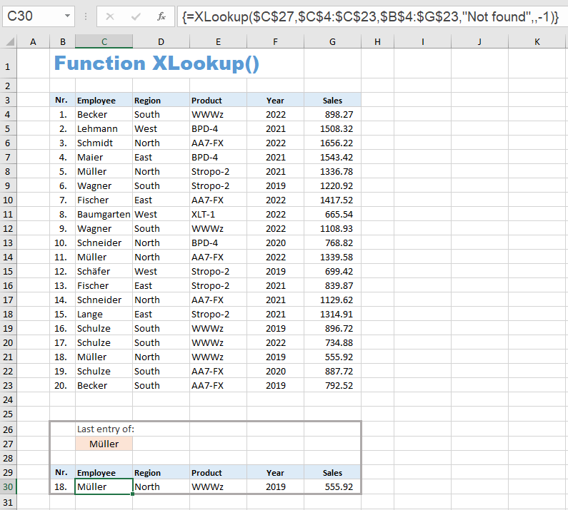
This example shows five of the new possibilities:
- Multiple values can be returned, not just one (here the six values in cells B30:G30).
- The address of a column is given instead of a column number. This column can therefore also be to the left of the search area.
- The list can also be searched in reverse order so that the last occurrence of the search item is found.
- Default for searching is now exact match.
- You can specify a string that will be returned instead of the error code if the search was unsuccessful.
Other innovations:
- You can choose whether to search an unsorted list (search mode 1 and -1) or a sorted list (search mode 2 and -2). Even with an unsorted list, the next larger or next smaller element is found.
- You can now also search for empty fields (leave first parameter unspecified).
- If a range on the spreadsheet - i. e. no array - is specified for the 'return_array' parameter, which is usually the case, the XLOOKUP function does not return the values found, but a corresponding cell reference.
This last point opens up a whole range of new possibilities, because now the XLOOKUP function can be used in other formulas at those places where cell references are expected.
Example 2
This example shows such a case. Two XLookup functions are used as parameters in the SUM function.
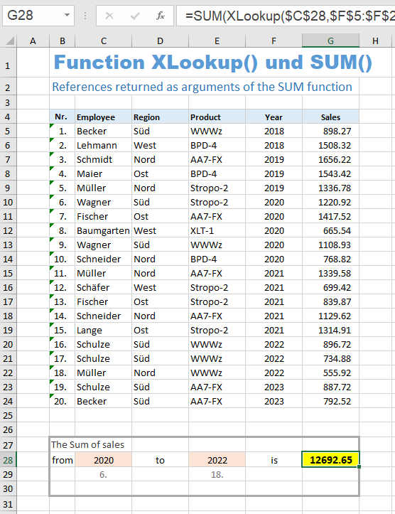
The formula in cell G28 is:
= SUM (XLookup ($C$28, $F$5:$F$24, $G$5:$G$24) : XLookup ($E$28, $F$5:$F$24, $G$5:$G$24, , ,-1)).
The prerequisite is that the year numbers are sorted in ascending order.
To calculate the sum of sales from 2020 to 2022, you can use the formula = SUM (G10:G22). To make the range variable, we replace the two addresses G10 and G22 with XLookup calls.
We replace the cell reference G10 with the expression XLookup ($C$28, $F$5:$F$24, $G$5:$G$24). The XLOOKUP function searches for the year 2020 in the normal search direction and therefore finds the first year 2020 in the 6th line of the list. It therefore returns the cell reference $G$10 from the return range $G$5:$G$24.
We replace the cell reference G22 with the expression XLookup ($E$28, $F$5:$F$24, $G$5:$G$24, , ,-1). The XLOOKUP function searches for the year 2022 in the opposite search direction and therefore finds the last year 2022 in the 18th line of the list. It therefore returns the cell reference $G$22 from the return range $G$5:$G$24.
Between the two XLOOKUP functions there is only the area colon, which makes an area from the two found addresses (G10 and G22) over which the SUM function sums. In this way you can now enter different years in the input fields C28 and E28 and always get the sum of sales for this period.
Additional note:
If the list of years is unsorted, you might consider replacing the second and third parameters in the XLOOKUP expressions with SORT(...). In this case you will get the error code #VALUE. This is because the SORT function does not return a cell reference, but an array of values. If the XLOOKUP function is passed an array instead of a cell reference, it does not return a cell reference but also an array. However, the SUM function requires cell references.
Example 2 shows this aspect of the XLOOKUP function (returning a cell reference) quite well. In practice, however, the task would still be solved using the SUMMEIFS function:
= SUMIFS ($G$5:$G$24, $F$5:$F$24, ">="&C28, $F$5:$F$24, "<="&E28)
This formula doesn't care if the years are sorted or not.
The search in an unsorted list has a speed disadvantage, because the search in a sorted list according to the so-called binary search method (search mode 2 or -2) is much faster.
Binary search works like number guessing, where you look for a number between 1 and 1000:
You choose the middle as the first number, i. e. 500, ask whether this is the number you are looking for and then you are told that the number you are looking for is larger. Then you choose the middle again from the range 501 to 1000, i. e. 750, and get the feedback that the number is smaller. If you continue this in the same way, you will have found the number you are looking for at the latest after 10 questions (and comparative feedback).
With an unsorted list of 1000 elements, you have to compare all values in the list one after the other (sequential search). In the worst case you have 1000 comparisons, on average about 500 comparisons.
Addition:
Function XLOOKUP2
The XLOOKUP2 function is not one of the functions available in Excel 365, but invented by me.
My motivation: A LOOKUP function with multiple search criteria is often asked on the Excel forums, and also a LOOKUP function that returns a list of all matches found.
The XLOOKUP2 function enables three things in addition to the XLOOKUP function:
- Multiple search criteria
- Wildcards in all search criteria (optional)
- Return of all matches found (optional)
The third item allows to filter data using wildcards (*, ?, ~) - see ▸Example 4 (Filtering with wildcards).
Syntax
= XLookup2 ( lookup_value1, lookup_array1, return_array, [if_not_found],
[match_mode], [search_mode],
[lookup_value2], [lookup_array2], [lookup_value3], [lookup_array3], ... )
| Parameter | Explanation |
|---|---|
| lookup_value1 | 1st search criterion |
| lookup_array1 | Array or range in which the 1st search criterion is searched (one-dimensional - single column or single row) |
| return_array | Array or range from which found values are returned |
| if_not_found (optional) |
Text returned in place of the #N/A error code if nothing was found |
| match_mode (optional) |
Match type: 0: Exact match search (default) 1: Invalid (generates the error #VALUE) -1: Invalid (generates the error #VALUE) 2: Search with wildcard symbols, the wildcards *, ?, ~ can be used for the search |
| search_mode (optional) |
Search mode: 1: Normal search order starting with the first item (default), the first match found is returned -1: Reverse search order starting with the last item, the first match found is returned 2: Normal search order, all matches are returned -2: Reverse search order, all matches are returned |
| lookup_value2 (optional) |
2nd search criterion |
| lookup_array2 (optional) |
Array or range in which the 2nd search criterion is searched (one-dimensional - single column or single row) |
| lookup_value3 (optional) |
3rd search criterion |
| lookup_array3 (optional) |
Array or range in which the 3rd search criterion is searched (one-dimensional - single column or single row) |
| etc. | . . . |
The first six parameters are identical to those of the function XLOOKUP.
The first two parameters are the 1st search criterion and the 1st lookup array. Any number of other pairs consisting of search criterion and lookup array can follow after the sixth parameter. Search criteria that are not specified or contain the empty string have no effect on the search.
It should be noted that the values 1 and -1 are invalid for the 'match_mode' parameter. The search for a next larger or next smaller value would no longer be unique if there were several search criteria. The values 0 and 2 have the same meaning as in XLOOKUP.
In the 'search_mode' parameter, the values 1 and -1 have the same meaning as in XLOOKUP, the values 2 and -2 have a different meaning than in XLOOKUP. A binary search in pre-sorted lists would no longer make sense with multiple search criteria - and thus multiple lists.
Example 3:
This example shows the search for the four search criteria employee, region, product and year.
Since nothing is entered for 'year', the fourth parameter does not limit the search result.
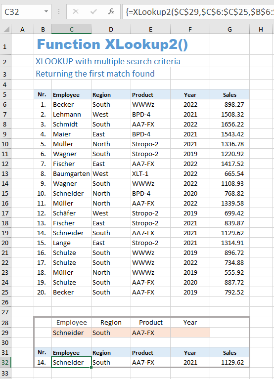
The formula used is:
= XLookup2 ($C$29, $C$6:$C$25, $B$6:$G$25, "nothing", 0, 1, $D$29, $D$6:$D$25, $F$29, $F$6:$F$25, $E$29, $E$6:$E$25)
The match_mode parameter is 0 (exact search), the search_mode parameter is 1 (normal search order, returning only the first match found).
Example 4 - filtering with wildcards
This example shows a search for the four search criteria employee, region, product and year with wildcards and returning all matches found.
The match_mode parameter is 2 (searching with wild cards). The search_mode parameter is 2 (return of all matches found and normal search order starting with the first item of the list).
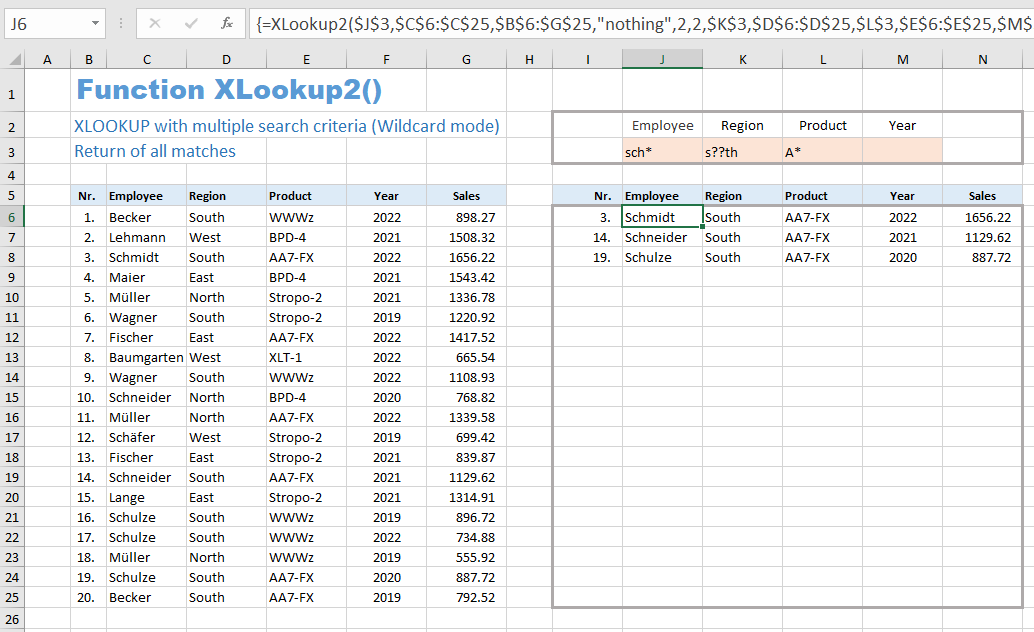
The formula used is:
= XLookup2 ($J$3, $C$6:$C$25, $B$6:$G$25, "nothing", 2, 2, $K$3, $D$6:$D$25, $L$3, $E$6:$E$25, $M$3, $F$6:$F$25)
With search_mode = -2 you would get the same search result, but in reversed order.
The range I6:N25 was preselected as the target range for this formula. This leaves enough space to, in extreme cases, also include the complete list as a result array.
The behavior of the XLOOKUP2 function in this example is identical to that of the FILTER function.
The only difference: In the XLOOKUP2 function, Wildcards (*, ?, ~) can also be used for filtering. This is not possible in the FILTER function.
Special topic:
The XLOOKUP function in array formulas
In an Excel forum I encountered a question for which no answer was found for good reason - at least not according to the ideas of the questioner. He wanted to know if there was a way to solve his problem with a single formula, with no intermediate results in hidden columns.
The solution would have been to make an expression with a VLOOKUP function an array formula by specifying an array of multiple search criteria instead of a single search criteria. This expression would then need to be used as an argument in a COUNTIF function.
The surprise:
When trying it out, I found that this solution formula didn't work due to a buggy or incomplete implementation by the Microsoft programmers in my Excel 2019! When I replaced the VLOOKUP function with XLOOKUP in Excel Online, it worked.
I would like to reproduce the situation with a simplified example:
The names of any three employees are entered in the I5:I7 range.
In cell K13, the sum of sales for these three selected employees should be displayed.
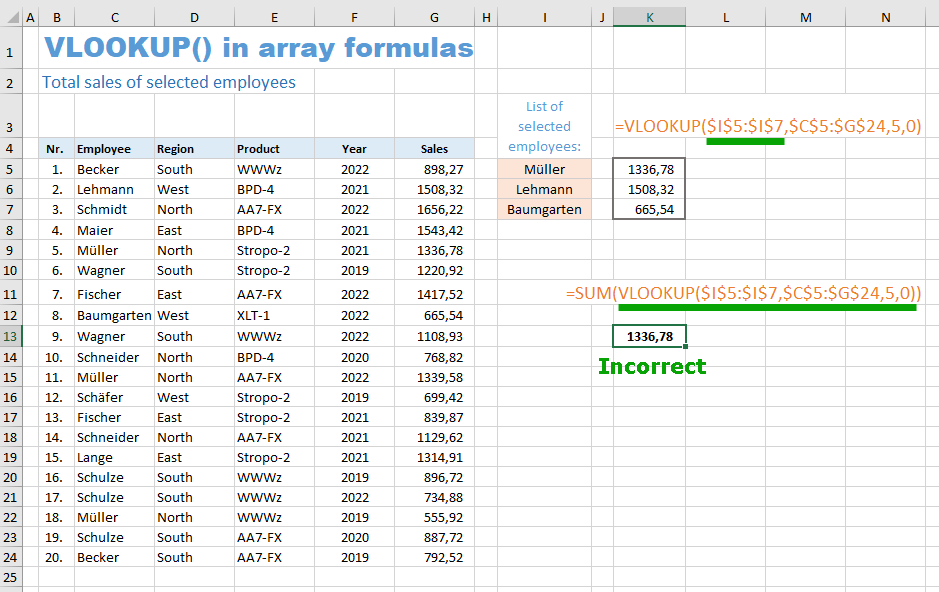
The area K5:K7 was selected, the formula = VLOOKUP ($I$5:$I$7; $C$5:$G$24; 5; 0) entered in the edit line and completed with CTRL-SHIFT-ENTER. The VLOOKUP function returns an array of three sales numbers represented in the range K5:K7.
Everyone who is familiar with array formulas expects that this 'intermediate result' in the range K5:K7 is not required, but that the VLOOKUP expression can be used as a parameter in a SUM function. This has been done in cell K13. But the SUM function doesn't get the correct list passed from the VLOOKUP function. Microsoft left a BUG and preferred to invest its manpower in subsequent versions.
The same example in online Excel using the XLOOKUP function works as expected:
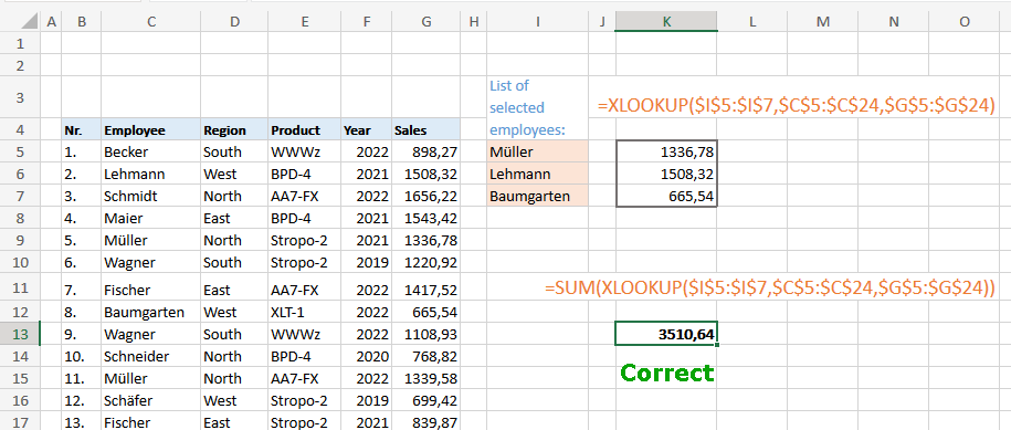
Working with this example, I realized that I completely forgot to program my UDF 'XLookup' in such a way that it can also process an array of several search criteria as the first parameter.
As of version 3.7 of the download file, this deficiency has been eliminated and the functions 'XLookup' and 'XCompare' can now also be used in array formulas.
I noticed another Microsoft BUG in the original XLOOKUP function:
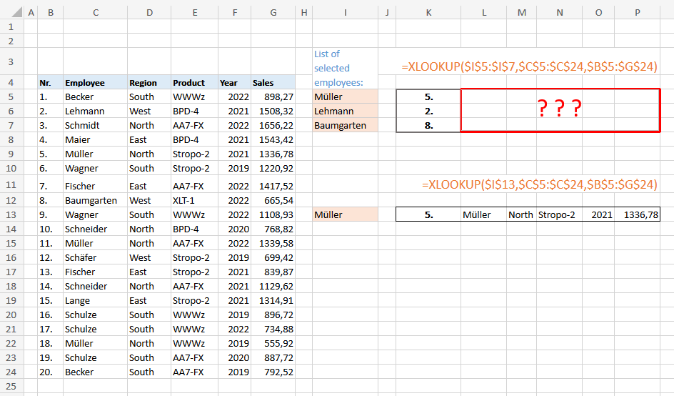
The third parameter of the XLOOKUP function, the return array, controls which columns of the found record are returned. In this example, the return array $B$5:$G$24 says that all columns from B to G should be returned. However, this only works with Microsoft if you are looking for a single record (formula in cell K13). If you search for several records (formula in cell K5), only the first column is returned for each hit.
At least in Excel-Online (tested on 06.01.2023) I get this effect. So I guess it's the same in Excel 365.
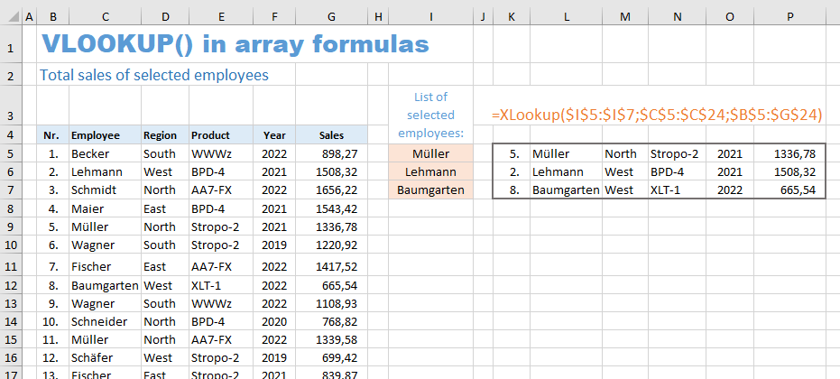
My UDF 'XLookup' returns all the columns:
For Excel 365 users
If you use Excel 365 and are interested in the two special functions SORTBY2 and XLOOKUP2, you can download an Excel file here that only contains these two UDFs:
▸Download Excel file
(Version 3.5 - Last update: 2024-10-24)
Tutorial: Create Excel UDF
Using the XLOOKUP2 function as an example, this tutorial shows how to create such a UDF with the help of VBA and which special things have to be considered. All phases from the evaluation of the parameters to the implementation of the search process and the processing of the return value are explained in detail.

Sharing knowledge is the future of mankind