
EXCEL function
FILTER
for Excel 2007 to 2019
Download the Excel file with the VBA code of the functions
SORT, SORTBY, FILTER, XLOOKUP, XMATCH, UNIQUE, SEQUENCE, RANDARRAY
and all examples shown on these web pages:
▸Download Excel file
(Version 3.8 - Last update: 2024-10-24 - XLookup and XMatch now fit for use in array formulas ▸more on this)
What is it about?
In Excel 365 and from Excel 2021, Microsoft implemented the long-missing cell functions SORT, SORTBY, FILTER, XLOOKUP and others. However, they were not retrofitted for older versions of Excel, so that all users from Excel 2007 up to and including Excel 2019 had to do without them.
There is now a solution for users of older versions of Excel (since the end of January 2022).
With the help of VBA so-called UDFs (user defined functions) were implemented that have exactly the same parameter lists as the corresponding Microsoft functions.
In cases where the functions provided here return multiple values, their input must be terminated with CTRL-SHIFT-ENTER. Before entering the formula, an area must be selected on the spreadsheet that contains the returned data - as is usual with the so-called CSE array formulas (CSE = Control Shift Enter).
▸This tutorial provides a basic and detailed introduction to array formulas.
With Function names of UDFs it doesn't matter whether the letters are written in upper or lower case.
For instructions on integrating the functions in your own Excel file, see ▸Integrating the functions.
FILTER function
If you are looking for a way to filter with wildcards, you can jump straight down to the ▸relevant chapter.
The Filter_ function is a replacement for the FILTER function which is only available in Excel 365. It expects exactly the same parameter list as the Excel 365 function and has the same filtering behavior.
The function name is "Filter_" with an underscore at the end because Excel does not accept the function name "Filter" as a name for a UDF.
= Filter_ ( array, filter criteria, [if_empty] )
| parameters | explanation |
|---|---|
| array | range or array to filter |
| filter criteria | An expression that produces a Boolean array whose length equals the height or width of the array to be filtered |
| if_empty (optional) |
A string that appears when the list of filtered dates is empty default: if_empty = "" |
See also the function description from Microsoft:
▸https://support.microsoft.com/en-us/office/filter-function-f4f7cb66-82eb-4767-8f7c-4877ad80c759
Example: = Filter_ ($B$3:$F$85, $F$3:$F$85>1000, "The filtered list is empty.")
In this example, the column F is used for filtering. From the range $B$3:$F$85, those rows are filtered out in with the value in column F is greater than 1000.
The function uses the (vertical) filter criterion $F$3:$F$85>1000 to recognize that vertical filtering is desired. This means that certain rows are filtered out.
Four more examples follow for illustration, which also show the combination of the functions Sort_ and Filter_ as well as the nesting of the Filter_ function (multiple filtering).
Filter - example 1
In this example horizontally is filtered. So certain columns are filtered out.
The filter criterion is: (B5:E5="Region") + (B5:E5="Sales")
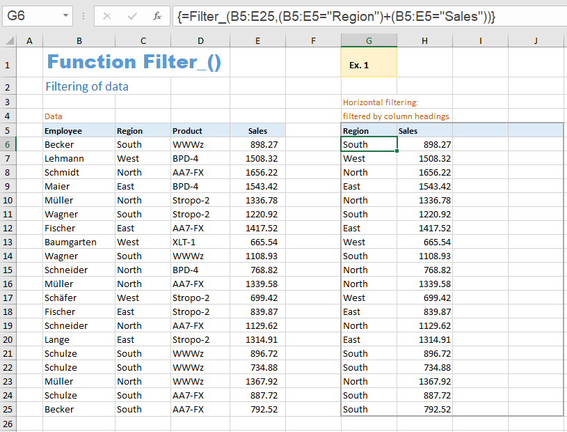
The columns 'Region' and 'Sales' are filtered out here.
RULE:
If several filter criteria are linked, they must be enclosed in brackets.
For the OR concatenation, the plus sign (+) is used, for the AND concatenation the multiplication operator (*) is used.
Since the dynamic adjustment of the output area cannot be simulated with VBA, you have to select a specific output area on the worksheet before entering the formula, as is usual with CSE array formulas. It is best to choose the same size as that of the original data.
Filter - example 2
In example 2 filtering is vertical, i.e. certain rows are filtered out.
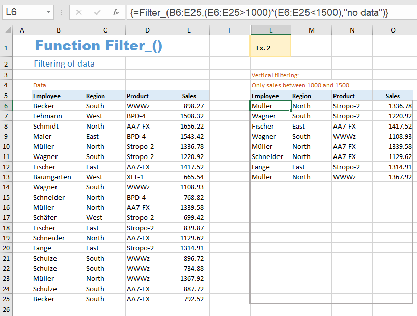
In this case, all those rows are filtered out in which column E has sales between 1000 and 1500.
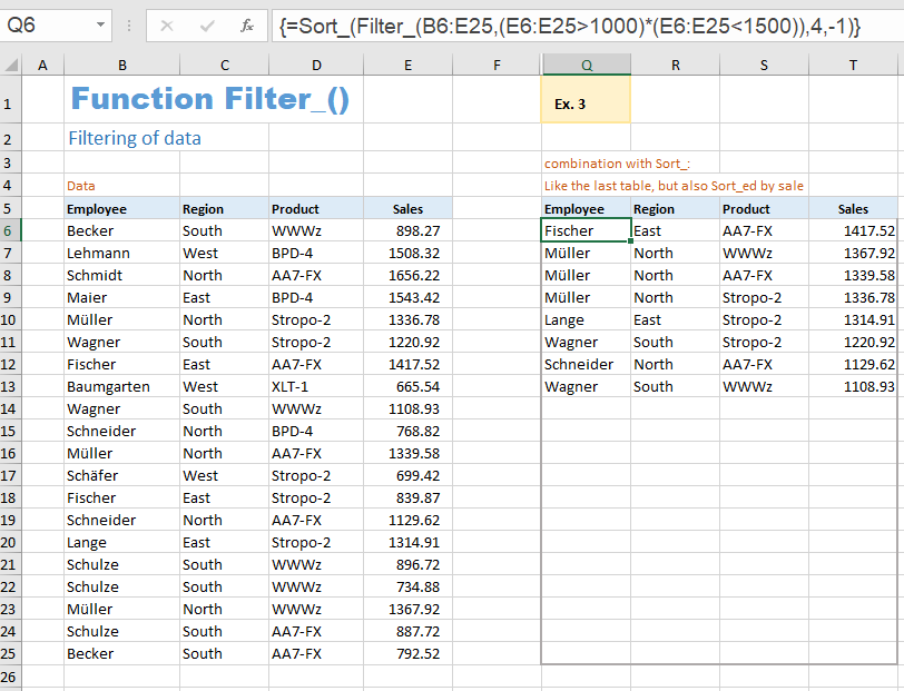
Filter - example 3
Example 3 shows how to combine the Sort_ and Filter_ functions. The filtered data from example 2 is also sorted by sales. To do this, you pass the complete filter expression of the previous formula as the first parameter to the Sort_ function.
Filter - example 4
Finally, an example for multiple filtering.
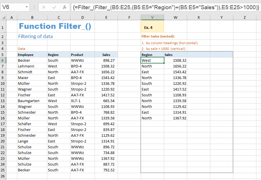
It is first filtered horizontally. The columns 'Region' and 'Sales' are filtered out. The second is vertical filtering. All sales greater than 1000 are filtered out.
The inner filter function of the formula filters the columns 'Region' and 'Sales' out. This whole inner filter expression is used in the outer filter function as the first parameter. The outer function takes over the result array of the inner function and filters it according to the column 'Sales'.
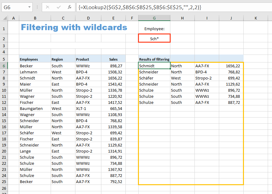
Filtering with wildcards
Unfortunately, Microsofts FILTER function does not support the use of wildcards (*, ?, ~) in the filter criteria.
However, if you are looking for a simple function for filtering with wildcards, you will find a solution in the XLOOKUP2 function. This function is not a built-in function of Excel, but a UDF (User Defined Function) programmed with VBA.
A small example file is intended to demonstrate the use of this function XLookup2 for filtering with wildcards:
▸Download the sample file for filtering with wildcards
In addition to the "XLookup2" function, the example file also contains the "Sort_", "Filter_", "XLookup" etc. functions for older versions of Excel mentioned at the top of this web page.
The formula used is:
=XLookup2($G$2,$B$6:$B$25,$B$6:$E$25,"",2,2)
The first parameter $G$2 is the search term. It can contain the wildcards * ? ~.
The second parameter $B$6:$B$25 is the column to search in.
The third parameter $B$6:$E$25 specifies the range from which the hits are returned.
A string can be specified in the fourth parameter, which will be displayed if the search is unsuccessful.
The fifth parameter "2" indicates that a search with wildcards takes place.
The sixth parameter "2" means to search in normal search order (first to last element) and return all matches, not just the first.
Hint:
Since this is a so-called array formula, the range G6:J25 must first be selected before entering the formula in the editing line. The entry of the formula must be completed using CTRL-SHIFT-ENTER.
Further information about the XLookup2 function and a more complex example for filtering with wildcards can be found here:
▸Example 4 - filtering with wildcards
Additional topic:
Filtering without FILTER function
How can you automatically filter data without the FILTER function - just by using conventional formulas?
Some people rely on such a solution if, for example, they use Excel 2019 or an older version and do not want to use macros.
The procedure will be shown and explained using a small example file. It can be downloaded here:
▸Example file for filtering without FILTER function
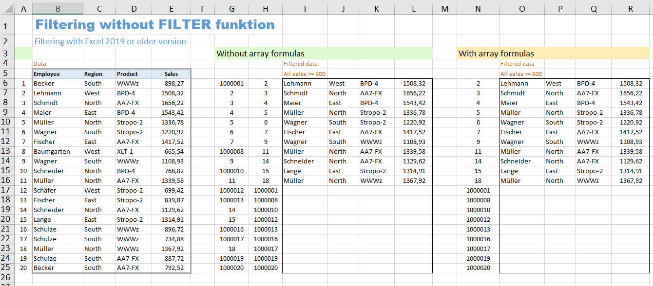
The starting material is the data in the range B6:E25. All rows with sales >= 900 should be filtered.
The example file presents two solutions: one without array formulas and a second with array formulas.
a) Solution without array formulas
In column A we first enter the consecutive numbers 1 to 20. This auxiliary column as well as the two following ones can be hidden later.
In cell G6 we enter the following formula:
=ROW(A1)+NOT($E6>=900)*1000000
This formula is copied down to cell G25.
The part of the formula shown in red (the argument of the NOT function) is the filter criterion. The formula generates consecutive numbers starting from 1 for all sales that meet the filter criterion. If the sales do not meet the filter criterion, the number 1000000 is added to the consecutive number. The aim of this is to ensure that these large numbers are all at the end of the list during subsequent sorting.
The subsequent sorting of the generated numbers is done using the formula:
=SMALL($G$6:$G$25,ROW(A1))
This formula is entered into cell H6 and copied down.
Using the VLOOKUP function, we can now display the rows with the small numbers. We enter the formula
=IFERROR(VLOOKUP($H6,$A$6:$E$25,2,0),"")
in cell I6 and copy it down.
The VLOOKUP function generates an error for the large numbers. The preceding IFERROR function ensures that an empty cell appears in these cases.
The formulas for the other three columns are:
Cell J6: =IFERROR(VLOOKUP($H6,$A$6:$E$25,3,0),"")
Cell K6: =IFERROR(VLOOKUP($H6,$A$6:$E$25,4,0),"")
Cell L6: =IFERROR(VLOOKUP($H6,$A$6:$E$25,5,0),"")
The red parameter decides which column of the original data should be displayed here.
b) Solution with array formulas
The auxiliary column with the sorted sequential numbers can be created with a single array formula. To do this, we mark the range N6:N25, enter the formula
=SMALL(ROW($1:$20)+NOT($E$6:$E$25>=900)*1000000,ROW($1:$20))
in the editing line at the top and complete the entry not with ENTER, but with CTRL-SHIFT-ENTER. The formula then automatically appears in the editing line in curly brackets.
NOTE:
If you want to use multiple filter criteria in this second variant, you cannot use the AND or OR function to link the filter criteria, but rather the operators * and +. A formula that filters out all sales from 900 to 1200 would then look like this:
=SMALL(ROW($1:$20)+NOT(($E$6:$E$25>=900)*($E$6:$E$25<=1200))*1000000,ROW($1:$20))
To display the filtered data, you can mark the range O6:R6 (the first row), enter the formula
=IF(N6>1000000,"",OFFSET($B$5:$E$5,N6,0))
in the editing line at the top and complete the entry with CTRL-SHIFT-ENTER.
This array formula is then copied down.
If you would like to familiarize yourself with array formulas, you can find a detailed introduction here:
▸Tutorial on array formulas
Sharing knowledge is the future of mankind