
EXCEL function
UNIQUE
for Excel 2007 to 2019
Download the Excel file with the VBA code of the functions
SORT, SORTBY, FILTER, XLOOKUP, XMATCH, UNIQUE, SEQUENCE, RANDARRAY
and all examples shown on these web pages:
▸Download Excel file
(Version 3.8 - Last update: 2024-10-24 - XLookup and XMatch now fit for use in array formulas ▸more on this)
What is it about?
In Excel 365 and from Excel 2021, Microsoft implemented the long-missing cell functions SORT, SORTBY, FILTER, XLOOKUP and others. However, they were not retrofitted for older versions of Excel, so that all users from Excel 2007 up to and including Excel 2019 had to do without them.
There is now a solution for users of older versions of Excel (since the end of January 2022).
With the help of VBA so-called UDFs (user defined functions) were implemented that have exactly the same parameter lists as the corresponding Microsoft functions.
In cases where the functions provided here return multiple values, their input must be terminated with CTRL-SHIFT-ENTER. Before entering the formula, an area must be selected on the spreadsheet that contains the returned data - as is usual with the so-called CSE array formulas (CSE = Control Shift Enter).
▸This tutorial provides a basic and detailed introduction to array formulas.
With Function names of UDFs it doesn't matter whether the letters are written in upper or lower case.
For instructions on integrating the functions in your own Excel file, see ▸Integrating the functions.
UNIQUE function
The Unique function is a replacement for the UNIQUE function which is only available in Excel 365. It expects exactly the same parameter list as the Excel 365 function.
= Unique ( array, [by_columns], [exactly_once] )
| parameter | explanation |
|---|---|
| array | The range or array from which to return unique rows or columns |
| by_columns (optional) |
A Boolean value that indicates whether to compare rows or columns TRUE: Columns are compared and returned FALSE: Rows are compared and returned (default) |
| exactly_once (optional) |
A Boolean value TRUE: All rows or columns that occur exactly once are returned FALSE: The duplicates are removed from the rows or columns (default) |
See also the function description from Microsoft:
▸https://support.microsoft.com/en-us/office/unique-function-c5ab87fd-30a3-4ce9-9d1a-40204fb85e1e
Depending on the value of the third parameter, this function fulfills two different tasks. If the third parameter is not specified or FALSE, all duplicates are removed from the rows/columns and each row/column is listed only once. If the third parameter is TRUE, all rows/columns that occur exactly once are selected. Rows/columns that occur more than once are thus completely omitted.
Matching two rows/columns means that all cells of the first row/column match the corresponding cells of the second row/column.
Examples of Unique
Here are some examples for using the Unique function, in the second example also the combination with Sort_.
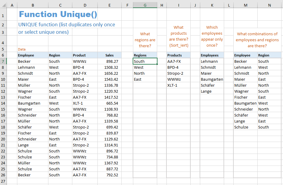
The formulas used are:
= Unique ($C$7:$C$26)
= Sort_ (Unique ($D$7:$D$26))
= Unique ($B$7:$B$26, , WAHR)
= Unique ($B$7:$C$26)
Example for the combination of Sort_, Filter_ and Unique
This example shows how to list all employees of region "South" in alphabetical order.
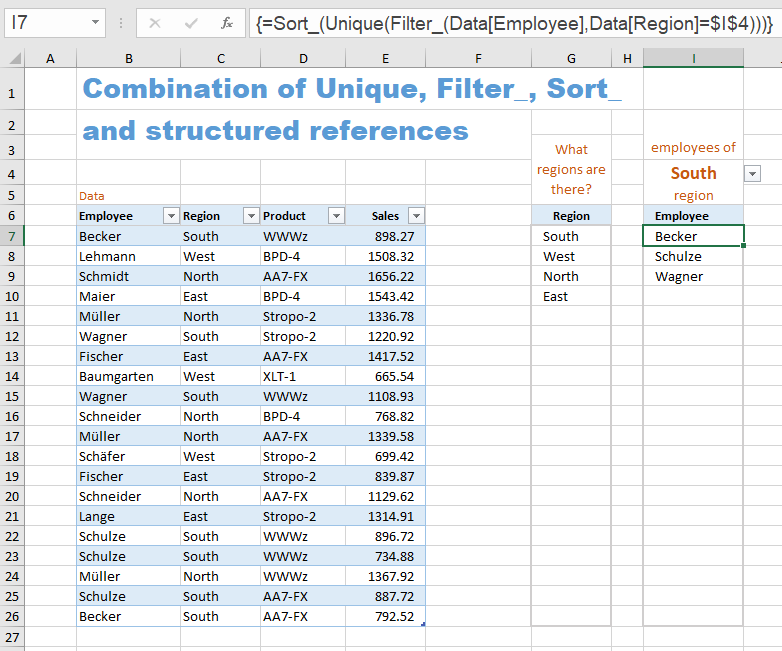
With the formula expression
Filter_ (Data[Employee], Data[Region]=$I$4),
all employees of the "South" region are first filtered out (in the drop-down selection field I4 the "South" region should be selected).
To ensure that no employee is listed more than once, the entire formula expression is inserted into the Unique function:
Unique (Filter_ (Tabelle[Mitarbeiter], Tabelle[Region]=$I$4)).
In order to sort the employee list, this second formula expression is used in the Sort_ function:
= Sort_ (Unique (Filter_ (Tabelle[Mitarbeiter], Tabelle[Region]=$I$4))).
Example: Total sales of all employees
This example determines the total sales for each employee.
The first list is sorted by employees, the second list by sales.
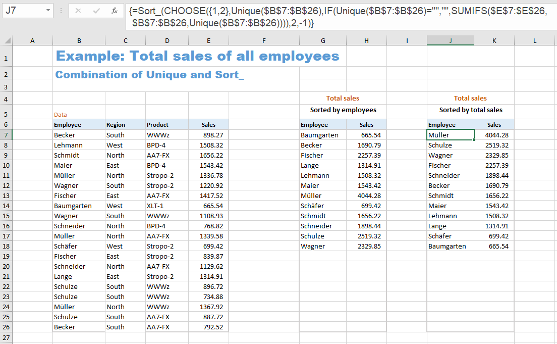
The first list consists of two formulas.
Column 'Employees':
{=Sort_ (Unique ($B$7:$B$26))}
The UNIQUE function returns the list of employees (each only once), and the SORT function sorts this list alphabetically.
Column 'Sales':
{=IF (G7:G26="", "", SUMIFS ($E$7:$E$26, $B$7:$B$26, G7:G26))}
With the help of the SUMIFS function, the total sales of the employees are determined.
The second list consists of a single formula:
{=Sort_ (CHOOSE ({1,2}, Unique ($B$7:$B$26), IF (Unique ($B$7:$B$26)="", "", SUMIFS ($E$7:$E$26, $B$7:$B$26, Unique ($B$7:$B$26)))), 2, -1)}
These formulas are explained in detail in the ▸Tutorial 'Array formulas' - Example 9.
For those interested who may not be able to use the UNIQUE and SORT functions because they are using an open source program there is added a conventional solution without these two functions:
Addition:
Total sales of all employees - conventional solution
In the image below, columns G through M are hidden.
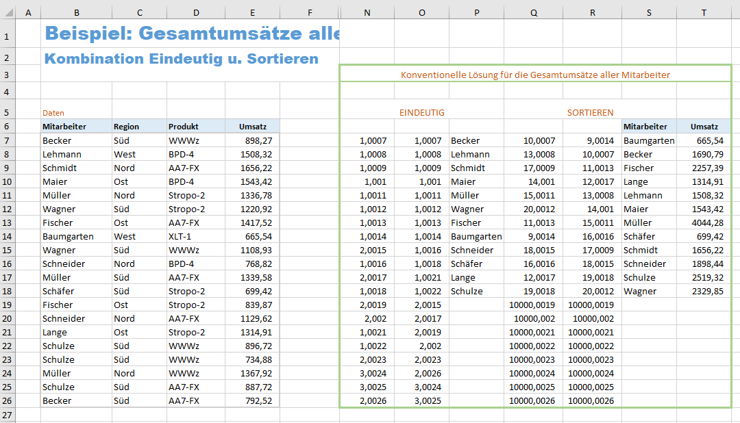
It is a solution for the case 'Sorted by employees' (first list).
The following formulas are used:
Cell N7:
=COUNTIF ($B$7:$B7, $B7) + ROW() / 10000
Cell O7:
=SMALL (N$7:N$26, ROW (A1))
Cell P7:
=IF (O7 > 2 ,"" ,INDEX ($B$7:$B$26, MATCH (O7, $N$7:$N$26, 0)))
Cell Q7:
=COUNTIF ($P$7:$P$26, "<=" & $P7) + ROW() * 0.0001 + ($P7 = "") * 10000
Cell R7:
=SMALL (Q$7:Q$26, ROW (A1))
Cell S7:
=INDEX ($P$7:$P$26, MATCH (R7, $Q$7:$Q$26, 0))
Cell T7:
=IF (S7 = "", "", SUMIFS ($E$7:$E$26, $B$7:$B$26, S7))
All seven formulas are copied down.
The individual formulas are also explained in detail in ▸Tutorial 'Array formulas' - section 9.3.
Sharing knowledge is the future of mankind