
Excel Tutorial
Array formulas
What is it?
This tutorial can also be downloaded as a PDF file:
▸Download the PDF file (Last update: 10.01.2023)
For this tutorial there is an Excel file with all examples for (free) download:
▸Download the Excel file with the examples (Last update: 08.09.2022)
Clarification of terms
1. What is an array?
If you have a list of numbers (e.g. 12, 15, 20, 22, 25), we like to talk about an array, and you can imagine this list of numbers in Excel arranged next to each other in a row or below each other in a column.
If one has an array of numbers that extends over multiple rows and multiple columns, one likes to speak of a two-dimensional array or a two-dimensional matrix. The number array (matrix) extends in two dimensions: to the right and downwards.
2. Old array formulas (CSE) - new dynamic array formulas
Since the September 2018 update, Excel 365 has the new so-called dynamic array formulas. Microsoft has classified the previous array formulas as obsolete. Excel 2021 also knows the new dynamic array formulas.
Until Excel 2019, there are only the non-dynamic ones, also called CSE formulas, because you do not finish entering the formula with Enter, but with Control-Shift-Enter. The difference between the two will be explained ▸below.
This tutorial was originally written on the subject of 'CSE array formulas', but its contents apply equally well to the new dynamic array formulas.
The array formulas should not be confused with the matrix functions. This refers to Excel functions that perform special mathematical calculations in connection with matrices, e.g. the multiplication of two matrices (MMULT) or the transposition of a matrix (TRANSPOSE).
What is an array formula?
A normal Excel formula determines a result or value (e.g. numeric result, date or text) and displays it in the cell where the formula is located. The formula is said to return a single value. An array formula returns a whole array of values. However, an array formula can also return a single value. And that brings us to the two cases to consider in connection with array formulas:
Case 1: The array formula returns multiple values (multi-cell array formulas).
Case 2: The array formula returns only one value (single-cell array formulas).
It's time for a first example!
Example 1: Array formula that returns multiple values
We open a blank Excel sheet and enter some simple numbers in the B3:D6 range.
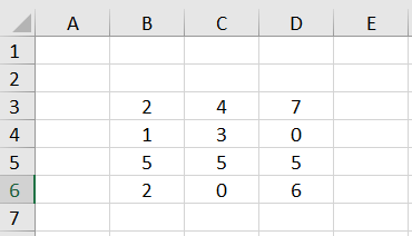
Thus we have a 4✕3 array of numerical values (4 rows and 3 columns).
If we would now enter the simple formula =B3*10 in cell F3, the result 20 would be displayed in F3. If we want Excel to use a single formula to multiply the entire array B3:D6 by 10 and return an array (a field of numbers) of results, then we can use the array formula =B3:D6*10. However, if we type this formula into the cell F3 and press ENTER, we get the error #VALUE.
We must follow two rules when entering (CSE) array formulas:
Rule 1:
If the array formula returns multiple results - in this case a 4✕3 array of numerical values, we need to select a corresponding 4✕3 range before entering the formula (so-called target range).
Rule 2:
The input of the formula must not be finished with the ENTER key, but with the key combination CTRL+SHIFT+ENTER. After that, Excel always displays this formula in curly braces to make it clear that this is an array formula - so in our example {=B3:D6*10}.
The braces must not be entered in the edit line! This would result in Excel interpreting the supposed formula as simple text.
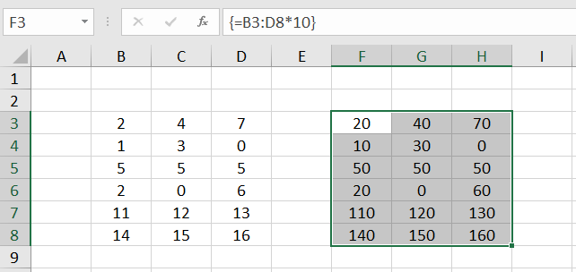
So we select the range F3:H6, enter the formula =B3:D6*10 in the edit line at the top and finish the input with CTRL+SHIFT+ENTER.
Excel calculates a 4✕3 number array of results - the so-called result array - and displays it in the F3:H6 range, the target range.
1.1 Parts of an array cannot be changed
If we now click on individual cells of our result array, we will always see the same array formula in the edit line at the top. An attempt to delete or change the content of a single cell within the result array is rejected by Excel with the message "You can't change part of an array".
Inserting a new blank row is also not possible if this blank row would run through the middle of the target range of an array formula.
To change the array formula, click any cell within the target range, change the formula in the edit line at the top, and press CTRL-SHIFT-ENTER to complete the change.
To use the F3:H6 cell range differently, you can first select it completely and then delete the content with the DEL key. Alternatively, you can click any cell within the target range, delete the formula in the edit line at the top, and complete the change with CTRL-SHIFT-ENTER.
1.2 The target range
The target range is the range you select before entering the array formula. In our example, we have chosen the range F3:H6 as the target range. Since the array formula returns a 4✕3 array, the target range also exactly matches the returned result array.
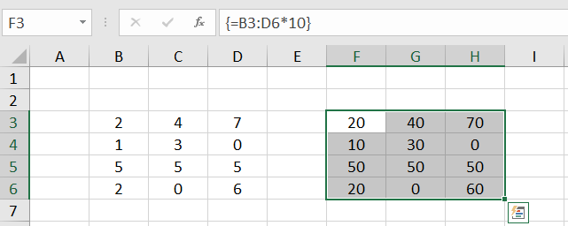
But what happens if the target range is smaller than the expected result array?
To investigate this, we delete the range F3:H6 again. We now select only the range F3:G4 and enter the array formula =B3:D6*10. The result looks like this:
Obviously, only the upper left part of the result array appears here in the target range. The rest is not displayed. This is referred to as an "intersection". By "intersection" we mean the intersection (i.e. the common or overlapping range) between the target range and the result array calculated by Excel.
This explains the initially frequent phenomenon of forgetting to select the target range before entering the array formula, and then finding that the top left value of the result array is displayed in the only cell that is now considered the target range.
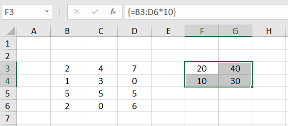
What happens now if the target range is selected too large?
We delete the previous array formula again and select as target range the range F3:F8:
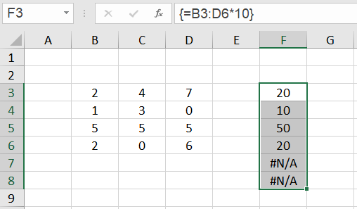
We see: According to the principle of intersection, the left column of the result array is displayed in the range F3:F6. In the cells F7 and F8 the error #N/A (no value available) appears. The error code #N/A always means that no valid value could be calculated for this cell. The occurrence of this error in array formulas is often an indication that the target range was selected too large.
1.3 Extension of the target range
We assume that our range of numbers has grown. Two more rows have been added. In order to adapt our array formula to the new situation, it is now not necessary to completely delete the old target range. We just need to select the new target range F3:H8, change the cell address D6 to D8 in the formula edit line at the top, and press CTRL+SHIFT+ENTER again.
Example 2: Array formula that returns only one value
For an array formula that returns only one value, no target range of several cells is preselected, but the array formula is entered into a single cell and the input is terminated with CTRL+SHIFT+ENTER.
Let's assume we want to multiply all the numbers in the range F3:H6 by 10 and sum the results. To do this, we enter the following array formula in cell F3:
=SUM (B3:D6*10)
and finish the input with CTRL+SHIFT+ENTER.
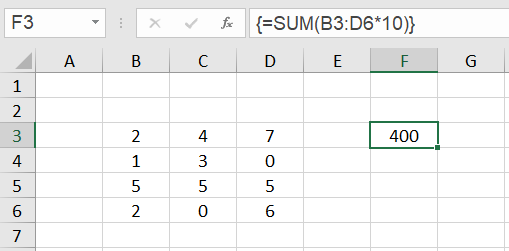
In the cell F3 the result 400 appears.
What happens here?
If we would only finish the input of the formula with ENTER, the error #VALUE! would be displayed in the cell F3. The SUM function expects cell addresses or constants as parameters and cannot do anything with the calculation expression B3:D6*10.
But if Excel is told by the key combination CTRL+SHIFT+ENTER that it is an array formula, the calculation expression B3:D6*10 is evaluated to a result array, exactly the one we see in the target range F3:H6 in example 1. The SUM function then adds up all the numbers in the result array.
2.1 Evaluate Formula - array constants
We can look at this process by selecting the cell F3, clicking Formulas ➝ Evaluate Formula in the menu bar at the top, and clicking 'Evaluate' in the window that opens.
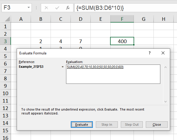
Now you see that the argument for the sum function is the expression
{20,40,70; 10,30,0; 50,50,50; 20,0,60}.
This is a so-called array constant. In these constants the elements of the first row are enumerated first and separated by a comma, then the elements of the second row follow and so on. The rows themselves are separated by a semicolon.
If the comma is set as a decimal separator in your regional settings, in the array constant the backslash is used as a separator instead of the comma.
Detailed information about array constants can be found for example ▸here.
Such an array constant is allowed as a parameter for the SUM function. If we were to type the formula =SUM ({20,40,70; 10,30,0; 50,50,50; 20,0,60}) directly into the edit line and conclude with ENTER as a normal formula, the formula would calculate the value 400 for us without complaint.
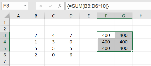
2.2 Target range too large
Array formulas that return only one value behave differently if the target range is selected too large, i.e. more than one cell is preselected. The error #N/A does not appear in the superfluous cells, but in this case the result of the array formula is displayed in all selected cells:
Array formulas that refer to multiple cell ranges
The array formulas considered so far only referred to a single cell range. For example, the formula {=SUM (B3:D6*10)} in example 2 referred to cell range B3:D6.
But what happens if there are several cell ranges in an array formula and they may have different extents?
To do this, we consider several cases in which an array formula has to process two different cell ranges. So that the whole thing is as transparent as possible, we take a simple addition of these two cell ranges.
Case 1:
In the simplest case, both cell ranges have the same extent. We enter the numbers 100,200,300, ... ,1200 in the B3:D6 range and the numbers 1,2,3, ... ,12 in the F3:H6 range. We select the target range B9:D12, enter the formula =B3:D6+F3:H6 in the editing line at the top and finish the input with CTRL+SHIFT+ENTER.
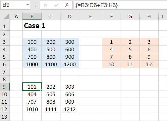
We can see from the result that the array formula returns a result array in which B3+F3, C3+G3, etc. are added together. So the result array has the form:
{B3+F3,C3+G3,D3+H3; B4+F4,C4+G4,D4+H4; B5+F5,C5+G5,D5+H5; B6+F6,C6+G6,D6+H6}
Adding two 4✕3 matrices again results in a 4✕3 array. That's exactly what we expected.
Case 2:
Next we add a 4✕3 array and a single cell, so a 1✕1 array. We select the target range B9:D12, enter the formula =B3:D6+F3 in the editing line at the top and close the input with CTRL+SHIFT+ENTER.
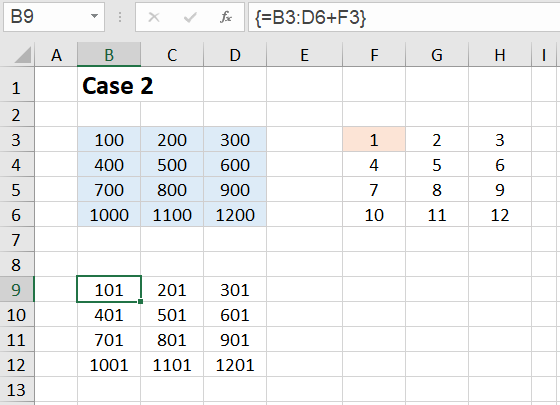
This second case does not surprise us either. The number 1 from cell F3 is added to each number in the range B3:D6. The result array has the form:
{B3+F3,C3+F3,D3+F3; B4+F3,C4+F3,D4+F3; B5+F3,C5+F3,D5+F3; B6+F3,C6+F3,D6+F3}
You get the same result if you add a 4✕3 array of all ones to the array in the range B3:D6.
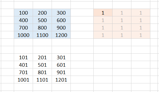
One can therefore also imagine that Excel internally expands the 1✕1 array to size 4✕3 and fills it with ones.
Case 3:
Now let's see what happens when we add a 4✕3 array and a 1✕3 array. We select the target range B9:D12, enter the formula =B3:D6+F3:H3 in the editing line at the top and close the input with CTRL+SHIFT+ENTER.
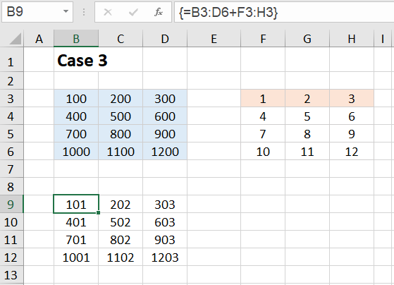
A 1 is now added everywhere in the first column, a 2 in the second column and a 3 in the third column. The result array has the form:
{B3+F3,C3+G3,D3+H3; B4+F3,C4+G3,D4+H3; B5+F3,C5+G3,D5+H3; B6+F3,C6+G3,D6+H3}
You get the same result if you add a 4✕3 array with 4 equal rows {1,2,3} to the array in the range B3:D6.
One can therefore also imagine that Excel internally expands the 1✕3 array to the size 4✕3 and fills the remaining rows with the values of the first row.
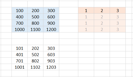
Case 4:
To be sure, let's try it with a single column as well. We add a 4✕3 array and a 4✕1 array. We select the target range B9:D12, enter the formula =B3:D6+F3:F6 in the editing line at the top and close the input with CTRL+SHIFT+ENTER.
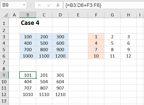
We see that in the first row a 1 is added everywhere, in the second row a 4, in the third row a 7 and in the fourth row a 10. The result array has the form:
{B3+F3,C3+F3,D3+F3; B4+F4,C4+F4,D4+F4; B5+F5,C5+F5,D5+F5; B6+F6,C6+F6,D6+F6}
You get the same result if you add a 4✕3 array with 3 equal columns {1;4;7;10} to the array in the range B3:D6.
And again you can imagine that Excel internally expands the 4✕1 array to the size 4✕3 and fills the remaining columns with the numbers from the first column.
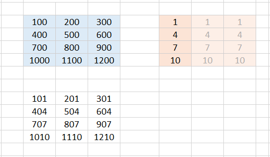
Case 5:
Yet another case works fine: we add a 1✕3 array and a 4✕1 array. We select the target range B9:D12, enter the formula =B3:D3+F3:F6 in the editing line at the top and close the input with CTRL+SHIFT+ENTER.
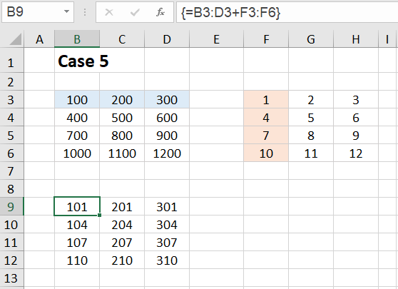
We see that the result array is again a 4✕3 array.
The result now looks as if Excel had expanded both matrices into a 4✕3 array - as shown in the following figure:
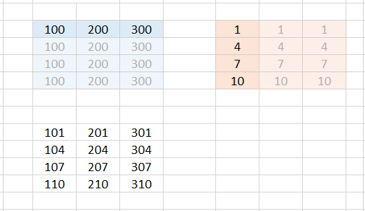
So you can also imagine that Excel internally expands both matrices into a 4✕3 array and fills it up by copying the row or column.
Case 6:
Finally, we consider one case as representative of the many other cases that lead to error messages. We're trying to add a 2✕3 array and a 4✕1 array. We select the target range B9:D12, enter the formula =B3:D4+F3:F6 in the editing line at the top and close the input with CTRL+SHIFT+ENTER.
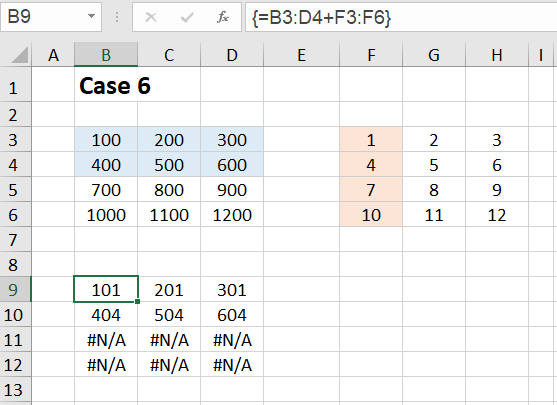
This time we get the #N/A error in the last two rows of the result array. For Excel, it is no longer clear with which content the last two rows of the extended array should be filled.
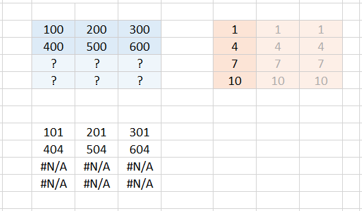
Apparently Excel can only fill in further rows if there is only one single row (see case 5). If there are already several rows, no more can be filled in automatically. The same applies accordingly to columns.
Summary:
If two cell ranges are to be calculated in an array formula that have a different number of rows or columns, you can imagine the evaluation of the formula in such a way that Excel internally expands both cell ranges to the same size. Additionally created rows (or columns) can only be automatically filled with values if only one single row (or one single column) is specified. Otherwise the error #N/A occurs in the target array.
Difference between old CSE formulas and new dynamic array formulas
For the new dynamic array formulas, unlike the old CSE array formulas, the following applies:
1. There is no need to preselect a target range. You enter the array formula in cell F3 and Excel determines the target range automatically. The result values flow from F3 to the right and down into the corresponding cells. If there are non-empty cells in this target range, the error code #OVERFLOW is displayed.
2. The formula input is completed - as with other formulas - only with the ENTER key. Excel automatically recognizes that it is an array formula.
3. If the range to which the array formula refers is increased or decreased, the target range is automatically adjusted. For example, if you delete a row in the range to which the array formula refers, the corresponding row in the target range is also automatically deleted. This is why the new array formulas are called 'dynamic'. The size of their target range or extension range adapts dynamically.
General information about the use of array formulas
To multiply all numbers in the range B3:D6 by 10, you certainly don't need an array formula. You could also enter the formula =B3*10 in cell F3 and copy it to the remaining fields.
But here already arises a first aspect to the use of array formulas. Let us imagine that we are not dealing with a 4✕3 range as in our example, but with a 4000✕3000 range, and all numbers are not multiplied by ten, but subjected to a more complex arithmetic operation. Here it would be advantageous to enter this formula as an array formula instead of copying it into 12 million cells. If one of these single formulas is changed by a carelessness, the error search is very tedious. With an array formula, it is not possible to accidentally change a single formula in the large number array. This source of error is, so to speak, excluded with an array formula.
Most examples given in connection with array formulas (here I mean the old CSE formulas) can be solved without an array formula. These introductory examples are often deliberately kept simple to make them easier to follow.
On the other side one reads: 'Array formulas make the impossible possible!'. However, I doubt this. What is possible with (CSE) array formulas can also be realized (in a roundabout way) with conventional formulas.
In my opinion, the calculations that run internally in a (CSE) array formula can always be broken down into individual steps, calculated with conventional formulas (e.g. in hidden areas), and the final result entered where the array formula would do it. In other words: What a (CSE) array formula can do, can also be realized by conventional formulas.
With the new dynamic array formulas, it may well be that the dynamic behavior and possibly other aspects cannot be reproduced by conventional formulas.
Of course, there is an increased space requirement, perhaps also a lower performance, but there is always space available on new empty Excel sheets (possibly hidden ones). Due to the additional formulas on the hidden auxiliary areas, there is certainly also a higher maintenance effort. In return, with space-saving, compact and sometimes ingenious array formulas, one accepts that they may be difficult to understand and require more time to analyze.
Let's look at some other examples.
Example 3: Copying a range
The simplest case for an array formula that returns multiple results is to copy an entire range. In this example, a copy of the range B2:D8 is created. In practice it can sometimes be desirable to make a certain range (an informative table) visible on another Excel sheet without being able to change individual values here. In our simplified example, the copied range appears directly below the original.
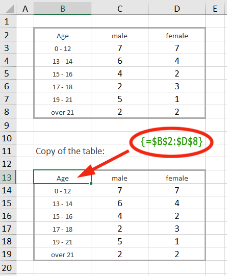
To create this copy, select a range of the same size - here the range B13:D19 - and enter the formula =$B$2:$D$8 in the edit line, terminating with CTRL+SHIFT+ENTER. The formula then appears in the edit line in curly braces: {=$B$2:$D$8}
In the copied range it is not possible to modify individual cells. You can only delete the range as a whole or change the formula for the entire range.
Example 4: Calculate total price
The following example is often used in connection with introductory examples for array formulas, although it is not really relevant in practice. It should not be missing here, because it illustrates in a simple way how an array formula works.
Examples where the use of array formulas is really appropriate very quickly lead to more complex formulas that are no longer transparent at first glance, as the last examples of this tutorial show.
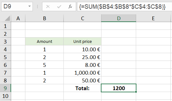
It is a simple calculation in which the amounts are multiplied by the individual prices and all results are added to a total price.
The SUM function expects single values or whole ranges as parameters.
With a calculation expression range * range - in our example $B$4:$B$8 * $C$4:$C$8 - it can't do anything and returns the #VALUE! error if you forget to finish the formula input with CTRL+SHIFT+ENTER.
However, if it is entered as an array formula using the CTRL+SHIFT+ENTER key combination, the formula evaluation runs differently. As can be seen by calling the menu item 'Evaluate Formula' (explained in more detail in ▶ Example 2.1), the calculation expression in the parenthesis is first evaluated to the array {10;50;40;1000;100} and then the SUM function is applied to this array.
This example is not very relevant in practice, because in practice the intermediate results would certainly be listed in column D and one then enters a simple sum formula in the cell D9.
The array formula becomes more interesting when several amount columns occur:
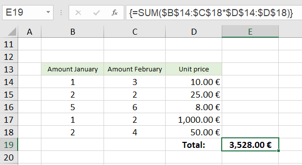
Here, the calculation expression $B$14:$C$18*$D$14:$D$18 is evaluated in such a way that all amount entries in column B as well as all amount entries in column C are multiplied by the unit prices in column D (compare ▶ Case 4 above). Two columns times one column results in a two-column array, in our example the array {10,30; 50,50; 40,48; 1000,2000; 100,200}.
The SUM function then adds the intermediate results of this two-column array to a total price in cell E19.
Example 5: Sum of the n largest numbers
From now on it gets more complex and the array formulas show their real strength.
To calculate the sum of the 10 largest numbers (n = 10) from a table of numbers, you could also show the ten largest numbers somewhere on the worksheet using the LARGE function without using an array formula, and place a simple summation formula underneath.
However, the use of an array formula is only really motivated if the number for n is not fixed, but is entered into a cell by the user of the worksheet. This case will be illuminated here.
This is what the whole thing looks like:
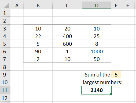
The cell D11 contains the formula:
{=SUM (LARGE ($B$3:$D$7, ROW (OFFSET ($B$1, , , $E$9))))}.
The formula calculates the sum of the n largest numbers from the array of numbers in the range B3:D7, where the value for the number n is read from the cell E9.
The best way to approach this formula is step by step.
5.1 First step
If we enter the formula =LARGE ($B$3:$D$7, 1) into the cell G3, we get the value 1000. This is the largest number of the number field.
For example, to get the second and third largest numbers, we could enter the formula =LARGE ($B$3:$D$7;2) below in cell G4 and the formula =LARGE ($B$3:$D$7, 3) in cell G5.
So that you don't have to type in five formulas for the five largest numbers, you resort to a little trick:
In the first formula (at the top), replace the 1 at the end of the formula with ROW(A1). The expression ROW(A1) also produces the number 1. But now you can copy the formula down, because in the second row ROW(A1) then becomes ROW(A2), in the third ROW(A3) and so on.
Instead of A1 you can also write B1 or X1. The column is irrelevant for the function ROW.
We try it out: We enter into the cell H3, the formula =LARGE ($B$3:$D$7, ROW(A1)). If we copy the formula down to cell H7, we get the five largest numbers displayed and can easily form the SUM.
BUT: The whole thing is not flexible. It is specified to the sum of five numbers.
5.2 Second step
We now proceed to an array formula. Instead of copying a conventional formula down several times, we select the range I3:I7, enter the formula =LARGE ($B$3:$D$7, {1;2;3;4;5}) in the edit line at the top, and finish by pressing CTRL+SHIFT+ENTER.
Since the second parameter of the LARGE function now does not consist of a single value, but of an array of five numbers, and the formula was declared as an array formula by the key combination CTRL+SHIFT+ENTER, the formula also returns an array of five results and distributes them over the selected range. We now see in the I3:I7 range the five largest numbers: 1000; 600; 400; 90; 50.
5.3 Third step
The next step is to let the function ROW generate the array {1;2;3;4;5}. We achieve this with the expression ROW (A1:A5).
We try it out: We select the range J3:J7, enter the formula =LARGE ($B$3:$D$7, ROW(A1:A5)) and finish with the key combination CTRL+SHIFT+ENTER. We see the five largest numbers again.
5.4 Last step
The last step is now that we construct a variable reference "A1:An" instead of the fixed reference A1:A5 for the function ROW.
Addresses for individual cells or also for entire cell ranges such as D4:F25 are also called references. They are what functions like SUM or ROW refer to, that is, they have these references as parameters. In the majority of cases, the functions return values (numeric values, date values, or texts). However, there are also functions that return references such as INDIRECT or OFFSET.
One of the functions that does not return a value but a reference is the OFFSET function. It has the syntax:
OFFSET (reference; rows; columns; [height]; [width])
The parameters mean:
-
reference:
Start value for the reference (single cell or range) -
rows:
Offset downwards or (for negative values) upwards -
columns:
Offset to the right or (for negative values) to the left -
height (optional):
Number of rows of the returned reference -
width (optional):
Number of columns of the returned reference
For example, the formula =OFFSET ($D$2, 1, 3, 4, 2) would return the reference G3:H6.
Starting from D2, we have an offset of one row down (D3) and 3 columns to the right (G3). So the upper left cell of the reference to be returned is G3. Since the height is to be 4 rows and the width 2 columns, the reference is G3:H6.
The formula =OFFSET ($A$1, , , 5) would return the reference A1:A5. The 'rows' and 'columns' parameters are not specified. Therefore they have the default value 0 (no offset downwards and no offset to the right). The 'height' parameter is specified as 5 and the optional 'width' parameter is missing; this thus has the value 1, because only a single cell is specified as the start reference ($A$1), which has the width 1. Starting from the initial value $A$1, we get a range of height 5 (i.e. 5 rows) and width 1 (i.e. 1 column) - we get A1:A5.
And with that we would have done it, because we only need to enter the cell address $E$9 instead of the 5 for the parameter 'height'. Then the number for the parameter 'height' is taken from this cell.
For example, if cell E9 contains the number 8, the expression OFFSET ($A$1, , , $E$9) creates the reference A1:A8, and the expression ROW (OFFSET ($A$1, , , $E$9)) is resolved to ROW (A1:A8), which in turn produces the array {1;2;3;4;5;6;7;8}.
The expression LARGE ($B$3:$D$7, ROW(OFFSET($A$1, , , $E$9))) is then resolved to LARGE ($B$3:$D$7, {1;2;3;4;5;6;7;8}) and this in turn to {1000; 600; 400; 90; 50; 25; 22; 20}.
The SUM function then forms the sum of these eight numbers.
Example 6: Alphabetical sorting
Here's a way to sort a list of names using a single array formula. - In Office 365 and from Office 2021 on, the new SORT function is available, which makes all these efforts superfluous.
STOP! - I have to stop here! This section is now obsolete. Since the end of January 2022, the SORT function has also been available for older Excel versions (Excel 2007 - Excel 2019)! It can be downloaded and used free of charge - see ▸hint at the bottom.
This would solve the following problem with the simple formula {= Sort ($B$4:$B$20) }.
However, if you want to study the structure of an array formula for sorting as a learning effect - or if you are using an open source product that does not run Microsoft VBA, you are recommended to read the rest of this section after all.
A prerequisite for the array formula presented here is that no name occurs twice. It is therefore particularly suitable for so-called IDs, i.e. combinations of letters, characters and digits that uniquely identify something, e.g. a sales item. The list to be sorted may have gaps.
The cell D4 contains the array formula
{=IFERROR (INDEX ($B$4:$B$20, MATCH (ROW ($A1), COUNTIF ($B$4:$B$20, "<="&$B$4:$B$20), 0)), "")}.
It was copied down to cell D20.
To understand the formula, let's first look at the sorting process without array formulas.
6.1 Sort without array formula
In the image below, columns D through I have been hidden.
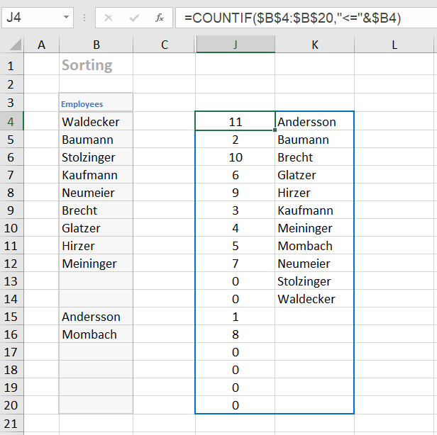
In cell J4 we enter the formula =COUNTIF ($B$4:$B$20, "<="&$B4) and copy it down to cell J20. This formula counts for each name in the list how many names are less than or equal to it. Thus, for each name we have a number that indicates the position of the name in the sorted list.
For example, the formula returns 11 for the name 'Waldecker' because all 11 names are less than or equal to 'Waldecker'. The value 2 is calculated for the name 'Baumann' because the two names 'Andersson' and 'Baumann' are less than or equal to 'Baumann' etc.
In the cell K4 we enter the formula =IFERROR (INDEX($B$4:$B$20, MATCH(ROW($A1), J$4:J$20, 0)), "") and also copy it down to the cell K20.
Let's look at this formula from the inside out. The expression ROW($A1) returns the number 1. When you copy it down, it becomes ROW($A2), ROW($A3) etc. That means it simply generates the numbers 1, 2, 3, ...
The MATCH function returns a relative position in a list. The expression MATCH (ROW ($A1); J$4:J$20; 0) in the first line is equivalent to the expression MATCH (1; J$4:J$20; 0). So the position of the '1' in the list J$4:J$20 is searched for. The '1' is found at position 12. Note that the alphabetically first name ('Andersson') is in the 12th position in column B. In the second line, the expression MATCH (2; J$4:J$20; 0) finds the number '2' in position 2. In the third line, the expression MATCH (3; J$4:J$20; 0) finds the number '3' at position 6. This means that the third name in alphabetical order ('Brecht') is in the 6th position.
The INDEX function now converts the position numbers found into the corresponding names. For example, the corresponding expression in the third line is INDEX ($B$4:$B$20; 6). So in the third line, the INDEX function gives us the name in the 6th position, namely 'Brecht'.
The innermost function ROW(...) produces the numbers 12, 13, 14, etc. from the 12th row, which produce an error in the formula. This error is caught by the outer function IFERROR. This function returns an empty string in case of an error.
6.2 Sort with multiple array formulas
For sorting without using an array formula one needs an auxiliary column in which the positioning of the individual names is determined. In the sorting formulas in the column K one accesses then these numbers, by inserting the reference J$4:J$20 as parameter of the function MATCH.
The idea now is to replace the reference J$4:J$20 with the function call that generates this list of positioning numbers and returns it as an array of 17 numbers. To do this, we take the formula in the J column, namely =COUNTIF ($B$4:$B$20, "<="&$B4) and replace the expression "<="&$B4) with "<="&$B$4:$B$20).
As a small intermediate experiment, we enter this new formula =COUNTIF ($B$4:$B$20, "<="&$B$4:$B$20) into the cell H4. Whether we finish the formula input with ENTER or with CTRL+SHIFT+ENTER, we always see only the first number, the 11. But if we select the H4:H20 range beforehand and then finish the formula input with CTRL+SHIFT+ENTER, we will see the whole list of numbers of the 17 positioning numbers.
If we now replace the reference J$4:J$20 in the conventional sort formula from column K with the function call COUNTIF ($B$4:$B$20, "<="&$B$4:$B$20) and finish the editing with CTRL+SHIFT+ENTER, we have created the array formula in cell D4. It returns the first name of the sorted list.
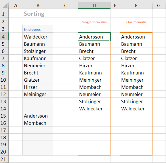
The array formula in cell D4 has been copied down. We therefore get seventeen individual, different array formulas in column D. The only difference between them is that in the middle of the formula the expression ROW(A1) becomes ROW(A2) in the next row and so on.
6.3 Sort with a single array formula
To get only one array formula for the whole column, we select e.g. the range F4:F20 and enter the same array formula, only instead of ROW(A1) we write ROW ($A$1:$A$17). We end the input with CTRL+SHIFT+ENTER. Now the whole range F4:F20 has the same array formula. Individual cells of this range can no longer be changed or deleted. So this solution is a little bit safer against an accidental change of single cells.
So the formula in cell F4 is:
{=IFERROR (INDEX ($B$4:$B$20, MATCH (ROW ($A$1:$A$17), COUNTIF ($B$4:$B$20, "<="&$B$4:$B$20), 0)), "")}
Example 7: VLOOKUP with multiple search criteria
In the cells G3 and G4 you can select two search criteria. The formula in cell G5 then finds the appropriate number of inhabitants from the table. The formula is:
{=VLOOKUP (G3&G4, CHOOSE ({1,2}, $B$4:$B$9&$C$4:$C$9, $D$4:$D$9), 2, 0)}
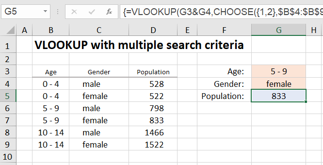
In the table above, if you want to search for the age group "5 - 9" using the VLOOKUP function to return the population for that age group, use the formula =VLOOKUP (G3, $B$4:$D$9, 3, 0)}.
The VLOOKUP function finds the first match in row 6 and returns the population 798. But it is also possible to search for the age group "5 - 9" and the gender "female".
To do this, use the string concatenation of both search criteria as the search criterion, in our case G3&G4.
Using the CHOOSE function, you create a table whose first column (the search column for the VLOOKUP function) consists of the string concatenations of the two columns B and C and whose second column consists of the column D with the population figures. The expression CHOOSE ({1,2}, $B$4:$B$9&$C$4:$C$9, $D$4:$D$9) returns exactly this table.
In this way you can also concatenate more than two search criteria with "&".
Example 8: Is my date of birth a prime number?
This final example really shows the power of array formulas. Its practical importance for the business world is zero, but it shows extraordinarily many aspects of the use of array formulas and is therefore very instructive.
In the first step it is shown how to test whether a given number is a prime number using a single (array) formula.
In the second step I present a possibility to calculate all factors of the number with the help of array formulas. However, in this case the formulas already become really complex.
8.1 Prime number test
First, let's look at how a number can be checked to see if it is a prime number.
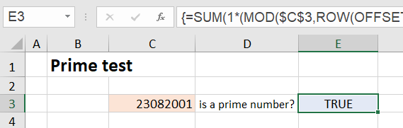
In cell C3 you enter the number to be checked, e.g. your eight-digit date of birth without the non-digits. The formula in cell E3 then checks whether it is a prime number. In the figure we see that 23.08.2001 (without the dots) is a prime number.
The (array) formula in cell E3 is:
{=SUM (1*(MOD($C$3, ROW (OFFSET ($A$1, , , INT (SQRT ($C$3)))))=0))=1}
The test method used here is mathematically very simple and not very optimized because this tutorial is not about prime number test methods, but about array formulas.
The number is divided by all numbers {1; 2; 3; 4; 5; ...} that are smaller than the root of the number. If the remainder of this division is zero, a factor of the number has been found. The outer function SUM in the formula determines the number of found factors. This number is equal to 1 for a prime number, since only once - namely when dividing by 1 - the remainder is equal to zero.
Explanation of the formula:
The expression ROW (OFFSET ($A$1, , , INT (SQRT ($C$3)))) generates the number array {1; 2; 3; 4; 5; ...; n}, where the last number n is equal to INT (SQRT ($C$3)), i.e. the largest integer that is still smaller than the root of the number to be tested. The generation of this number array is explained in detail in ▸section 5.4.
For example, the square root of 23082001 is equal to 4804.373, in which case the number array {1; 2; 3; 4; 5; ...; 4804} is generated. Our total formula looks like this after this calculation step:
{=SUM (1*(MOD($C$3, {1;2;3;4;5;...;4804})=0))=1}.
The MOD function calculates the remainder of an integer division. For example, the formula =MOD (27, 8) would return the value 3. In our case, the function MOD ($C$3, {1;2;3;4;5;...;4804}) returns the array of all remainders, namely {0;1;1;1;...;3585}. After the MOD function follows the expression =0, i.e. all numbers in the array of the remainder values are checked for equality with zero, and an array consisting of TRUE and FALSE values results.
Multiplication by 1 converts the TRUE and FALSE values to ones and zeros. So the SUM function returns the number of ones and thus the number of factors. If SUM (...)=1, there is a prime number.
8.2 Determination of all factors of a number
The factors of a number are obtained with an array formula that looks like a horror formula at first glance, and I sympathize with anyone who stops reading at this point.
The formula is:
{=IF (ROW()-5>SUM (1*(MOD ($C$3, ROW (OFFSET ($A$1, , , INT (SQRT ($C$3)))))=0)), "", LARGE ((MOD ($C$3, ROW (OFFSET ($A$1, , , INT (SQRT ($C$3)))))=0) * ROW (OFFSET ($A$1, , , INT (SQRT ($C$3)))), SUM (1*(MOD ($C$3, ROW (OFFSET ($A$1, , , INT (SQRT ($C$3)))))=0))-ROW (OFFSET ($A$1, , , INT (SQRT ($C$3))))+1))}
However, if you read on anyway, you will find that the outer scope of the formula is deceptive and the formula is not at all as complex as it looks.
It will, if you omit the outer IF function (function to intercept error codes) for now, reduce to a simple LARGE function. It has thus the structure =IF (..., "", LARGE (..., ...)). The LARGE function then returns the factors sorted by size.
How do you come up with such a formula?
8.2.1 Preliminary consideration with practical experiments
First, we consider how the factor search could be done at all (without array formulas). Let's take the number 20 as an easy-to-manage example.
We could divide the number 20 by all the numbers from 1 to 20 in order and see which divisors have a remainder of zero. These divisors are then the factors of the number 20.
Since the factors occur in pairs (i.e., for 20: 1-20, 2-10, 4-5), it is sufficient to check those factors that are less than or equal to the root of 20, in our case the numbers from 1 to 4. The factors paired with them can then be calculated by simple divisions NUMBER/FACTOR.
So that the whole thing does not remain a gray theory, let's solve the small example with the number 20 on the Excel sheet.
In cell C3 we enter the number 20.
In the cells G6:G9 we enter the numbers from 1 to 4. These are our divisors, which are to be checked to see if they are factors of 20.
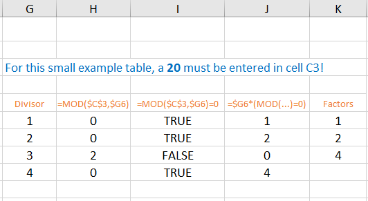
Since the MOD function of Excel =MOD (number, divisor) gives us directly the remainder of the division, we enter the formula =MOD ($C$3, $G6) into the cell H6 and copy it down to the cell H9. We get the remainders {0;0;2;0}.
Attention: In ($C$3, $G6) there is no dollar sign in front of the 6!
In the next column we convert the remainders into TRUE/FALSE values. TRUE means that there is a factor here. In cell I6 we enter the formula =MOD ($C$3, $G6)=0 and copy it down to cell I9.
In cell J6 we enter the formula =$G6*(MOD($C$3, $G6)=0) and copy it down to cell J9. In the J column we have all divisors which are factors of 20. At the places of the others a zero is generated.
Now comes the final work of the LARGE function: it lists the factors according to size - without the zeros in between. In the cell K6 we enter the formula =LARGE ($J$6:$J$9, 3), in the cell K7 the formula =LARGE ($J$6:$J$9, 2) and in the cell K8 the formula =LARGE ($J$6:$J$9, 1).
Your insides have probably already responded to these formulas with a shake of the head, because they are specialized to the number 20 and already fail when we enter the number 25 in C3. The next step has to be to generalize this special solution.
First, we will consider the transition to array formulas for this purpose.
Instead of entering three individual formulas as in the K column, we select the three cells L6:L9 and enter the formula =LARGE ($J$6:$J$9, {3;2;1}). This time we finish the input with CTRL+SHIFT+ENTER.
The behavior of the array formula in the L column is the same as that of the formulas in the K column: By the array {3;2;1} the third largest factor is determined in the first row, the second largest in the second row and the largest in the third row.
Our goal is to get at an array formula that does not require cached number sequences.
The main effect of using array formulas is that extensive intermediate results are not saved on the Excel sheet, but are calculated internally during the formula evaluation and immediately processed further.
The formula in the L column still uses the results in the J column. Therefore we look at how these results were calculated and insert the corresponding calculation expression into our array formula. So in our array formula we replace the reference $J$6:$J$9 with the calculation expression $G6*(MOD($C$3, $G6)=0). - But stop!
This calculation expression calculates only the first value. We need a calculation expression tailored to array formulas, that returns an array of all four values in the J column! In two places in this expression, we therefore replace the $G6 with $G$6:$G$9. Our new array formula is then:
=LARGE ($G$6:$G$9*(MOD ($C$3, $G$6:$G$9)=0), {3;2;1})
To test the formula, we select the cells M6:M8, enter the formula in the edit line, and close the input again with CTRL+SHIFT+ENTER.
If we now replace the reference $G$6:$G$9 in both places in the formula with the array {1;2;3;4}, we have an array formula that does not need any cached results at all. Its only reference is cell C3, where the number to be checked is located.
To test the formula, we select the range N6:N9 and enter the formula
=LARGE ({1;2;3;4}*(MOD ($C$3, {1;2;3;4})=0), {3;2;1}) <F0>.
Finish with CTRL+SHIFT+ENTER!
So much for the preliminary consideration. - We now know what the structure of the array formula must look like, but it must not be specialized to case 20.
8.2.2 Generalization of the previous array formula
If we look at the last array formula, we see that in two places we must generate a sequence of numbers from 1 to n, where n is the integer that is just less than the root of the number to be tested. The calculation of n is done by the calculation expression INT (SQRT ($C$3)).
The generation of a series of numbers of variable length is again done with ROW (OFFSET ($A$1, , , n)). The generation of this series of numbers is explained in detail in ▸section 5.4. For n we insert the arithmetic expression INT (SQRT ($C$3)) and get:
ROW (OFFSET ($A$1, , , INT (SQRT ($C$3)))) <F1>
So this calculation expression generates a number array of the shape {1;2;3;...;n} up to a last number n, which depends on the number to be checked. For the number 20 in our preliminary consideration, n = 4.
Besides this number array, we only have to create one more: At the end of the formula, we have to replace the array {3;2;1} with a number sequence that starts with the number of factors below the root value and then runs down. For the number 20, the number of factors below the root of 20 was equal to 3.
We would get this number 3 if we counted the number of zeros in the H column in our small example in the previous section 8.2.1. This counting is done with the array formula =SUM (1*(MOD ($C$3, {1;2;3;4})=0)).
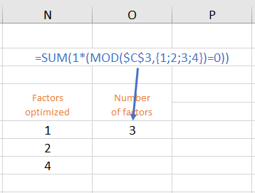
To understand this formula, you can display the formula evaluation in Excel. We enter the formula as an array formula in cell O6. The step-by-step formula evaluation results in:
SUM(1*(MOD(20, {1;2;3;4})=0))
SUM(1*({0;0;2;0}=0))
SUM(1*({TRUE;TRUE;FALSE;TRUE}))
SUM({1;1;0;1})
3
If we replace the expression {1;2;3;4} again as above with the generalized expression
ROW (OFFSET ($A$1, , , INT (SQRT ($C$3)))),
we get the calculation expression for determining the number of factors we are looking for:
SUM (1*(MOD ($C$3, ROW (OFFSET ($A$1, , , INT (SQRT ($C$3)))))=0)) <F2>
To get the descending sequence of numbers {3;2;1} at the end of the formula <F0>, we create an arithmetic expression of the form NumberOfFactors-{1;2;3;...;n}+1.
For example, if the number of factors is 15, the arithmetic expression is then evaluated as {15;14;13;12;11;...}.
For 'number of factors' we use the arithmetic expression we just developed and for {1;2;3;...;n} we use the arithmetic expression <F1>.
We get the arithmetic expression for the descending sequence of numbers:
SUM (1*(MOD ($C$3, ROW (OFFSET ($A$1, , , INT (SQRT ($C$3)))))=0))-ROW (OFFSET ($A$1, , , INT (SQRT ($C$3))))+1 <F3>
We are now ready to replace the three series of numbers (green) in the formula <F0> from Section 8.2.1 with the generalized arithmetic expressions <F1> and <F3>.
The formula
=LARGE ({1;2;3;4}*(MOD ($C$3, {1;2;3;4})=0), {3;2;1})
changes to:
=LARGE (<F1>*(MOD ($C$3, <F1>)=0), <F3>)
We will spare ourselves the confusing full text of this formula at this point.
That could now be the final formula. But due to the fact that the list of divisors <F1> (in the example {1;2;3;4}) is longer than the list of factors, the descending list <F3> (in the example {3;2;1}) goes from a certain point to zero and into the minus numbers. The LARGE function then outputs the error code #N/A (no value available).
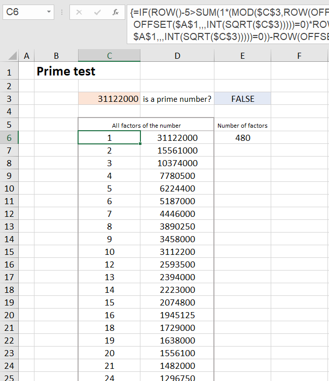
This error code could still be intercepted with IFNA. However, the IFNA function has no effect if a #N/A error is output because the target range of the array formula was selected too large. However, so that all the factors are output for numbers with a lot of factors (e.g. 31122000 with 480 factors), we have to select the target range large enough, although the next number 31122001, for example, only has 4 factors.
In order not to have hundreds of #N/A error codes on the Excel sheet in this case, we put an IF function in front of the already very confusing overall formula:
=IF (ROW()-5>NumberOfFactors, "", ...)
Since the first row of the target range of our array formula is row 6, the number 5 must be subtracted from ROW() so that the count starts at 1. If you move the target range up or down, the number 5 must be adjusted accordingly.
For example, the number 31122000 has the last factor found (the 240th) in row 245; the error code #N/A is generated in row 246. Since ROW()-5, i.e. 246-5, is greater than 240 (number of factors), the IF function ensures that an empty string ("") is written into the cell.
Our final overall formula looks like this:
=IF (ROW()-5><F2>, "", LARGE (<F1>*(MOD ($C$3, <F1>)=0), <F3>))
Or - because it looks so great - again in the full text:
{=IF (ROW()-5>SUM (1*(MOD ($C$3, ROW (OFFSET ($A$1, , , INT (SQRT ($C$3)))))=0)), "", LARGE ((MOD ($C$3, ROW (OFFSET ($A$1, , , INT (SQRT ($C$3)))))=0) * ROW (OFFSET ($A$1, , , INT (SQRT ($C$3)))), SUM (1*(MOD ($C$3, ROW (OFFSET ($A$1, , , INT (SQRT ($C$3)))))=0))-ROW (OFFSET ($A$1, , , INT (SQRT ($C$3))))+1))}
We enter the conventional formula =IFERROR ($C$3/C6, "") in cell D6 and copy it down to cell D305. A maximum of 600 factors can be displayed in the range C6:D305. Since the number 31129999 is the maximum that can occur with an eight-digit date of birth, this is sufficient in any case. In the number range from 1 to 3112999 there can be a maximum of 480 divisors.
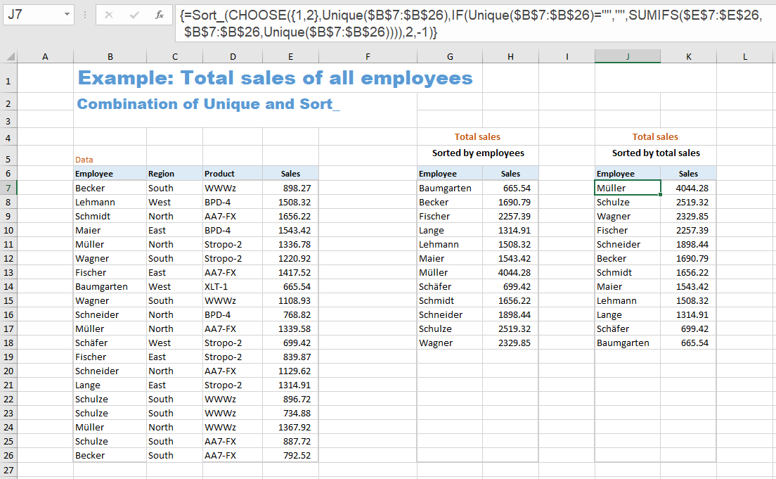
Example 9: Total sales of all employees
This example determines the total sales for each employee.
The first list is sorted by employees, the second list by sales.
In this example, the functions 'SORT' and 'UNIQUE' are used. These functions are not yet available in the older Excel versions up to and including Excel 2019. However, for the Excel versions from Excel 2007 to Excel 2019 one can download an implementation of these functions as UDFs (User Defined Functions) - see link at the bottom of this webpage.
For this reason, this example 9 cannot be found in the Excel example file for this tutorial, but in the Excel example file for the UDFs (worksheet 'Example Sales').
9.1 First List
The first list consists of two formulas.
Column 'employees':
{=Sort_ (Unique ($B$7:$B$26))}
The UNIQUE function returns the list of employees (each only once), and the SORT function sorts this list alphabetically.
The name of the UDF for sorting is 'Sort_'.
Column 'sales':
{=IF (G7:G26="", "", SUMIFS ($E$7:$E$26, $B$7:$B$26, G7:G26))}
In this column you could also enter the formula =SUMIFS ($E$7:$E$26, $B$7:$B$26, G7) in the first cell (H7) and copy it down. Then you wouldn't have an array formula, but a single formula in each cell. A preceding IF function suppresses the zeros in the blank lines:
=IF (G7="", "", SUMIFS ($E$7:$E$26, $B$7:$B$26, G7))
The transition to an array formula for the entire column is now done by using the range G7:G26 instead of G7 in two places in the formula. This gives you the formula
{=IF (G7:G26="", "", SUMIFS ($E$7:$E$26, $B$7:$B$26, G7:G26))}
9.2 Second List
The second list consists of a single formula:
{=Sort_ (CHOOSE ({1,2}, Unique ($B$7:$B$26), IF (Unique ($B$7:$B$26)="", "", SUMIFS ($E$7:$E$26, $B$7:$B$26, Unique ($B$7:$B$26)))), 2, -1)}
If you want to sort the list by sales, things get a little more complicated.
The solution idea is the following:
Using the CHOOSE function, we create a two-column matrix with the employees and their sales and sort this matrix with a preceding SORT function.
{=Sort_ (CHOOSE ({1,2}, Column_1, Column_2), 2, -1)}
The penultimate parameter (2) means that the 2nd column is used for sorting. The last parameter (-1) has the effect of sorting in descending order.
For Column_1 we use the expression Unique ($B$7:$B$26). It creates the unsorted list of employees.
The expression for Column_2 has the same structure as the array formula for the second column in the first list. This read:
{=IF (G7:G26="", "", SUMIFS ($E$7:$E$26, $B$7:$B$26, G7:G26))}
Since we now no longer have a reference column G7:G26, we must replace the range expression G7:G26 with the expression Unique ($B$7:$B$26) in the two relevant places.
For Column_2 we therefore use the following:
IF (Unique ($B$7:$B$26)="", "", SUMIFS ($E$7:$E$26, $B$7:$B$26, Unique ($B$7:$B$26)))
This results in the overall formula:
{=Sort_ (CHOOSE ({1,2}, Unique ($B$7:$B$26), IF (Unique ($B$7:$B$26)="", "", SUMIFS ($E$7:$E$26, $B$7:$B$26, Unique ($B$7:$B$26)))), 2, -1)}
In the older Excel versions (Excel 2019 and older) you have to select the entire target range J7:K26 before entering this formula and complete the entry of the formula with CTRL-SHIFT-ENTER.
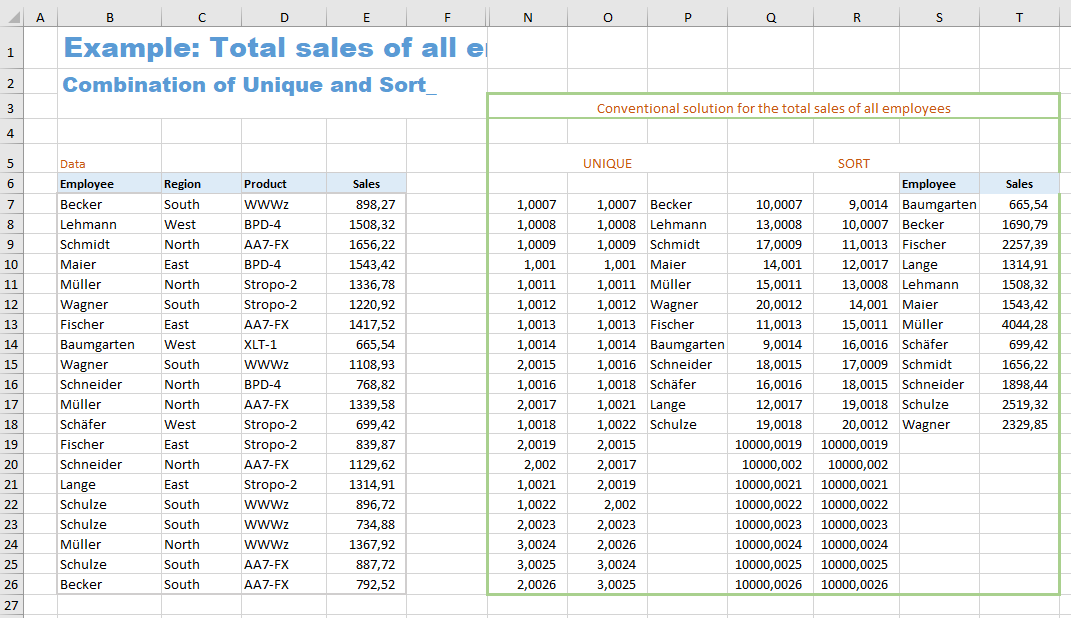
9.3 Complemental description: Total sales of all employees - conventional solution
Some may ask how such a list of total sales could be realized without the two functions UNIQUE and SORT and without array formulas. Or some are dependent on such a conventional solution because they are using an open source program that does not provide these functions. Therefore, this alternative solution is also considered here.
This is a solution for the case 'Sorted by employees' (first list).
Several auxiliary columns are required (columns N to R) which can be hidden later.
The formulas in the N, O, and P columns first create a list of all employees, in which each one appears only once. The formulas in the Q, R, and S columns sort this employee list. The sales of the individual employees are then totaled in column T.
The formula in cell N7 is:
=COUNTIF ($B$7:$B7, $B7) + ROW() / 10000
In the parameters of the COUNTIF function, it is crucial that $B7 appears twice without a dollar sign in front of the 7. If this formula is copied down, this function call becomes
COUNTIF ($B$7:$B8, $B8),
COUNTIF ($B$7:$B9, $B9),
etc.
In the 9th line, the expression COUNTIF ($B$7:$B15, $B15) generates a 2, because the name 'Wagner' occurs twice in the range $B$7:$B15. In this way, ones are generated the first time a name occurs, but higher numbers are generated for repeated occurrences of a name. In the next step, all names for which a one was generated are then transferred to column P.
So that the MATCH function can later find the position of these names unambiguously, a small fraction of the line number is added to each number. So each name has a unique identifier, and all names whose identifier is less than 2 are transferred to column P.
The formula in cell O7 is:
=SMALL (N$7:N$26, ROW (A1))
The expression ROW (A1) becomes ROW (A2) in the next line. The first line is the smallest number, the second line is the second smallest, and so on.
The function SMALL sorts the numbers from column N in ascending order. In this way, the numbers less than 2 (and thus the names occurring for the first time) come up to the top of the list.
The formula in cell P7 is:
=IF (O7 > 2, "", INDEX ($B$7:$B$26, MATCH (O7, $N$7:$N$26, 0)))
In the two columns B and N one can clearly see which name belongs to which identifying number. So we can now replace the sorted numbers in the O column with the associated names.
The new XLOOKUP function can do it, but the VLOOKUP function unfortunately cannot: looking up a value to the left of the search column. The combination of the two functions INDEX and MATCH has become established as a replacement for this lookup.
For each number in the O column, the MATCH function finds its relative position in the range N7:N26. For example, it finds the number 1.0021 in column N at position 15. The INDEX function then finds the name 'Lange' in column B at position 15. In the cell P17 the corresponding name 'Lange' appears to the right of the number 1.0021.
The IF function ensures that an empty cell appears in place of the names that appear for the second or third time.
Next step is sorting of this list of names. Here it is important to ensure that the empty cells in the list of names do not appear at the beginning of the list, but at the end.
The formula in cell Q7 is:=COUNTIF ($P$7:$P$26, "<=" & $P7) + ROW() * 0.0001 + ($P7 = "") * 10000
With this COUNTIF function, it is also crucial for the right effect that there is no dollar sign in front of the 7 in the second parameter "<=" & $P7. In the next line, the decision criterion for the count is then "<=" & $P8 etc.
For each name, the number of names less than or equal to it is counted. The first name 'Becker' has 10, namely the eight empty cells, the name 'Baumgarten' and the name 'Becker' itself. So each name gets a number that indicates its position in the sorted list. The name 'Becker' would be in the 10th position after the empty cells and the name 'Baumgarten'.
Again, we need to add a small fraction of the line number to this number so that the list of numbers is unique. In addition, we add the calculation term ($P7 = "") * 10000. Since in Excel TRUE = 1 and FALSE = 0, in case of an empty cell in column P, the expression ($P7 = "") will equal TRUE (returns the value 1) and thus adds the number 10000. This has the effect that the empty cells get the highest numbers and appear at the end of the list when sorted.
The formula in cell R7 is:
=SMALL (Q$7:Q$26, ROW (A1))
The numbers in the Q column are sorted in ascending order (just like in the O column).
The formula in cell S7 is:
=INDEX ($P$7:$P$26, MATCH (R7, $Q$7:$Q$26, 0))
This formula now looks up which name corresponds to the relevant number in column R. Here, as in column P, the combination of INDEX and MATCH is used again. An alphabetically sorted list of all employees is created.
The formula in cell T7 is:
=IF (S7 = "", "", SUMIFS ($E$7:$E$26, $B$7:$B$26, S7))
With the help of the SUMIFS function, the total of sales for each employee is calculated in column S. The IF function at the beginning of the formula means that empty cells instead of zeros appear after the last employee.
* * *
Hint:
Functions SORT, XLOOKUP, FILTER and others also for older Excel versions
The Excel 365 exclusive functions SORT, XLOOKUP, FILTER, UNIQUE and others have been available since the end of January 2022 also for users of Excel 2007 - Excel 2019. They were programmed as so-called UDFs (User Defined Functions) in the programming language VBA. They have exactly the same parameter lists as the Microsoft versions too. They are CSE array functions (CSE = Control Shift Enter) whose input must be completed with CTRL SHIFT ENTER.
More information and download are available here:
▸https://hermann-baum.de/excel/hbSort/en/
Sharing knowledge is the future of mankind