
EXCEL function
SORT
for Excel 2007 to 2019
Download the Excel file with the VBA code of the functions
SORT, SORTBY, FILTER, XLOOKUP, XMATCH, UNIQUE, SEQUENCE, RANDARRAY
and all examples shown on these web pages:
▸Download Excel file
(Version 3.8 - Last update: 2024-10-24 - XLookup and XMatch now fit for use in array formulas ▸more on this)
What is it about?
In Excel 365 and from Excel 2021, Microsoft implemented the long-missing cell functions SORT, SORTBY, FILTER, XLOOKUP and others. However, they were not retrofitted for older versions of Excel, so that all users from Excel 2007 up to and including Excel 2019 had to do without them.
There is now a solution for users of older versions of Excel (since the end of January 2022).
With the help of VBA so-called UDFs (user defined functions) were implemented that have exactly the same parameter lists as the corresponding Microsoft functions.
In cases where the functions provided here return multiple values, their input must be terminated with CTRL-SHIFT-ENTER. Before entering the formula, an area must be selected on the spreadsheet that contains the returned data - as is usual with the so-called CSE array formulas (CSE = Control Shift Enter).
▸This tutorial provides a basic and detailed introduction to array formulas.
With Function names of UDFs it doesn't matter whether the letters are written in upper or lower case.
For instructions on integrating the functions in your own Excel file, see ▸Integrating the functions.
SORT function
The SORT function allows you to sort specific areas on the spreadsheet. One or more column numbers/line numbers indicate which columns/lines should be sorted.
The function name is "Sort_" with an underscore at the end because Excel does not accept the function name "Sort" as a name for a UDF.
Syntax
= Sort_ (array, [sort_index], [sort_order], [by_column])
| parameters | explanation |
|---|---|
| array | range or array to sort |
| sort_index (optional) |
Number of the row or column to sort by (default: sort_index = 1) |
| sort_order (optional) |
Sort order 1 for ascending (default) -1 for descending |
| by_column (optional) |
FALSE for vertical sorting in the column (default) TRUE for horizontal sorting in the row |
The function behaves like the Excel 365 function SORT.
Also compare Microsoft's description of the function:
▸https://support.microsoft.com/en-us/office/sort-function-22f63bd0-ccc8-492f-953d-c20e8e44b86c
For example: = Sort_ ($B$3:$F$85, 3, -1)
The last parameter is missing. As a result, the default value FALSE is taken and it is sorted vertically (in the column). The range B3:F85 is sorted by the 3rd column (column D) in descending order.
What Microsoft doesn't document is the ability to sort by multiple criteria as well. You can also specify an array of column numbers instead of a single column number.
Example: = Sort_ ($B$3:$F$85, {4,3,1}, {-1,1,1})
Sorting is done according to columns 4 (descending), 3 (ascending) and 1 (ascending).
SORTBY function
The function SORTBY allows sorting by one or more sorting criteria.
Syntax
= Sortby (array, [by_array1], [sort_order1], [by_array2], [sort_order2], ... )
| parameters | explanation |
|---|---|
| array | range or array that to sort |
| by_array1 | range or array to sort by |
| sort_order1 (optional) |
Sort order 1 for ascending (default) -1 for descending |
| by_array2 (optional) |
range or array to sort by |
| sort_order2 (optional) |
Sort order 1 for ascending (default) -1 for descending |
The function behaves like the Excel 365 function SORTBY.
Also compare Microsoft's description of the function
▸https://support.microsoft.com/en-us/office/sortby-function-cd2d7a62-1b93-435c-b561-d6a35134f28f:
For example: = Sortby ($B$3:$F$85, $C3:$C85, -1, $E3:$E85, 1, $B3:$B85, -1)
The range B3:F85 is first sorted by column C in descending order (first sorting criterion). The second and third sorting criterion are columns E (ascending) and B (descending).
In this second parameter list, the columns that are sorted by can also be outside the range to be sorted - for example, on another worksheet.
There is no limit to the number of sorting criteria (consisting of one pair by_array and sort_order each).
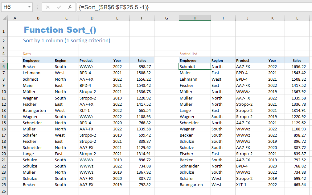
Sorting Example 1 - Sort by a single sorting criterion
The following example shows how to sort an employee list by Sales in descending order. The formula used is:
= Sort_ ($B$6:$F$25, 5, -1)
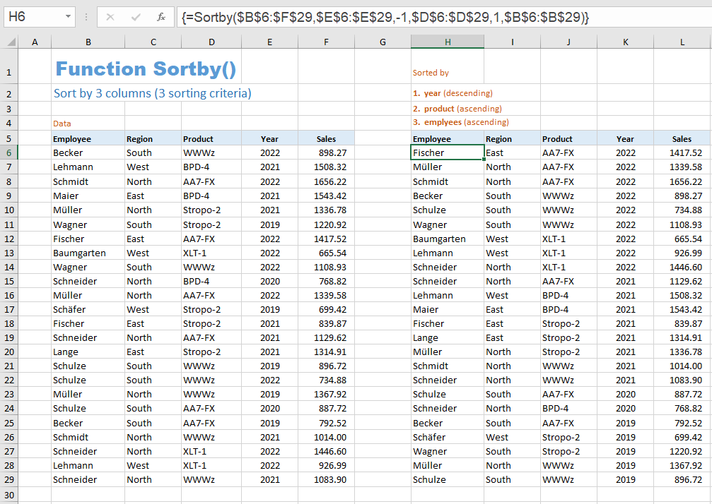
Sorting Example 2 - Sorting by multiple sorting criteria
The following example shows how to sort an employee list by year (descending order), within a year by product (ascending order), and within of a product by employees (ascending order). The formula used is:
= Sortby ($B$6:$F$29, $E$6:$E$29, -1, $D$6:$D$29, 1, $B$6:$B$29)
Specification
As already shown in the example above, it is possible to specify an array of numbers for the 'Index' parameter in the Sort_ function. These numbers must be row or column numbers that refer to rows or columns within the range to be sorted. Otherwise the error code #VALUE is returned.
With the Sortby function, the parameters by_array1, by_array2, ... must be single-column or single-line areas whose length corresponds to the corresponding dimension of the first parameter. If the length is too short, the #value error is returned. If it is too long, the superfluous cells are ignored.
Optional parameters at the end of the parameter list can be omitted entirely. In the middle of the parameter list, optional parameters can be omitted by just setting the parameter's comma.
The following two examples sort the range A1:A9 in descending order:
= Sort_ (A1:A9, , -1) first parameter list
= Sortby (A1:A9, A1:A9, -1) second parameter list
All parameters that expect a range address also accept a corresponding array or an expression that returns such an array. For example, the following call is possible too:
= Sortby ($B$6:$B$11, {4;2;1;3;5;6}).
The second parameter is then the first sorting criterion and defines a fixed (static) order. The first name in column B (the name in cell B6) appears in fourth position, the second in second position, the third in first position, and so on.
The dynamic spilling of the values into the neighboring cells depending on the space requirement, as it takes place in Excel 365, unfortunately cannot reproduced with VBA as a matter of principle. A user-defined function (UDF) programmed with VBA must return an array of values as the last action. Where the returned values are then distributed is no longer in the hands of the programmer, but is controlled internally by Excel.
A touch of dynamics can still be achieved if you convert the data to be sorted into a ▸table, so that you can use the so-called structured references in the parameter list of the Sort_ function. A small example is presented in the following section.
Use of structured references
A certain dynamic adjustment of the sorted area to an enlargement or reduction of the original data can be achieved if the original data is converted into a table and in the parameter list of the function Sort_ uses structured links.
In the example below, the initial data in the range B4:C10 has been turned into a table named 'Fond'. The range E5:F14 was selected, the formula = Sort_ (Fond) was entered in the editing line and the entry was finished with CTRL SHIFT ENTER.
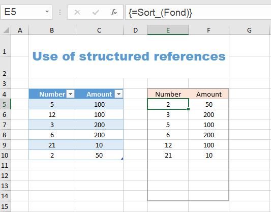
The range E5:F14 was deliberately chosen too large. In the range E11:F14, error codes #NV now appear. With the help of the conditional formatting =isNV(E5) and font color white, these error codes are hidden.
If the table of the original data is now expanded downwards or truncated upwards, the table of the sorted data is automatically expanded or truncated as well.
Addition:
Sortby2 function
The SortBy2 function doesn't exist in Excel 365. It's a real bonus. It has the same parameter list as Sortby.
In contrast to Sortby, it has an additional effect. For example, when sorting vertically and using multiple sorting criteria, the column with the first sorting criterion is displayed first (far left), followed by the column with the second sorting criterion, and so on, and then the remaining columns follow.
Sortby2 - Example 1
Example 1 shows sorting according to three sorting criteria: year, product and employee. With normal sorting (with the Sortby function), the same order of the columns would appear in the result area as in the area of the original data. So the first column would be 'Employees'. When using the Sortby2 function, on the other hand, the year is in the first column, the product in the second, etc.
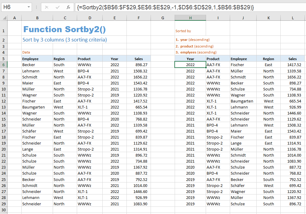
The Sortby2 function therefore displays the columns in the order of the sorting criteria. The same applies to horizontal sorting.
Sortby2 - Example 2
With the help of the Sortby2 function, the following scenario is possible without much effort:
- The original data can be sorted by any column, which means in this example by five sorting criteria.
- Any order of the sorting criteria is possible with the help of five selection fields (drop-down lists).
- The individual columns are always displayed in the order of the sorting criteria.
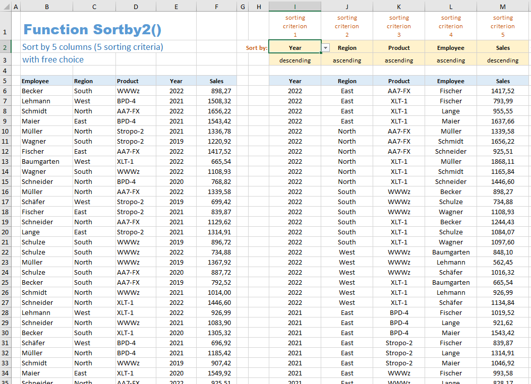
To sort by the five criteria of year, region, product, employee and sales, we can use the formula
= Sortby2 ($B$6:$F$105, $E$6:$E$105, -1, $C$6:$C$105, 1, $D$6:$D$105, 1, $B$6:$B$105, 1, $F$6:$F$105, -1).
But that would have fixed the order of the sorting criteria. Using the example of the first sorting criterion, we shall now show how this order can be made variable.
If the column heading 'Year' is selected in the I2 selection field, the fourth column of the original data should be used as the first sorting criterion. Instead of the fixed expression $E$6:$E$105 we need a variable expression that returns exactly this range.
The OFFSET function is the right choice here. The expression OFFSET ($B$6, 0, 3, 100, 1) would give us exactly the right range, but would still be not variable.
The first three parameters of the OFFSET function determine the upper left corner of the returned range. From $B$6 you move 0 rows down and 3 columns to the right. So the top left corner would be cell $H$6. The last two parameters specify the height and width of the returned area. So with a height of 100 and a width of 1, exactly the 'Year' column of the original data would be returned.
Apparently, we have achieved our goal if we calculate the third parameter (shift of the upper left corner to the right) depending on the text in cell I2. This is exactly what the expression MATCH ($I$2, $B$5:$F$5, 0) -1 does. The MATCH function looks for the word 'year' in the $B$5:$F$5 range (our column headings) and returns the column index 4. We subtract 1 and we're done.
We put the MATCH function as the third parameter in the OFFSET function and get the expression
OFFSET ($B$6, 0, MATCH($I$2, $B$5:$F$5, 0) -1, 100, 1).
In the last step, we insert this expression as the second parameter in the Sortby2 function. The other sorting criteria are also replaced by this expression, only we adjust the address of the selection field accordingly. Instead of $I$2, the second sorting criterion contains $H$2, etc.
The parameters that determine the sorting direction (ascending, descending) are replaced by IF functions:
IF($I$3="descending", -1, 1).
$I$3 becomes $H$3 for the next parameter, etc.
= Sortby2 ($B$6:$F$105, OFFSET($B$6, 0, MATCH($I$2, $B$5:$F$5, 0) -1, 100, 1), IF($I$3="descending", -1, 1), OFFSET($B$6, 0, MATCH($J$2, $B$5:$F$5, 0) -1, 100, 1), IF($J$3="descending", -1, 1), OFFSET($B$6, 0, MATCH($K$2, $B$5:$F$5, 0) -1, 100, 1), IF($K$3="descending", -1, 1), OFFSET($B$6, 0, MATCH($L$2, $B$5:$F$5, 0) -1, 100, 1), IF($L$3="descending", -1, 1), OFFSET($B$6, 0, MATCH($M$2, $B$5:$F$5, 0) -1, 100, 1), IF($M$3="descending", -1, 1))
![]()
Ready!
To relax you have a nice little problem: the birthday list.
Birthday list
You have a list with the columns Name and Birth date. From this list you would now like to create a birthday list that goes from January 1st to December 31st.
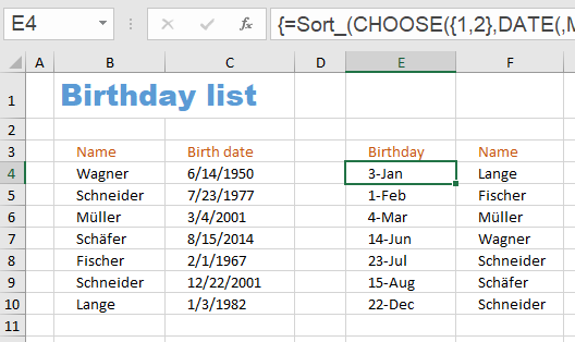
The formula is:
= Sort_ (CHOOSE({1.2}, DATE(, MONTH(C4:C10), DAY(C4:C10)), $B$4:$B$10))
The Sort_ function is called with a single parameter. It is the array returned by the CHOOSE function. The CHOOSE function creates an array consisting of two columns.
The first column is what the expression DATE(, MONTH(C4:C10), DAY(C4:C10)) returns. The first parameter of the DATE function is missing. This gives all date values the year 1900. All birthdays therefore have the year 1900 and are therefore sorted in the desired order. So that the year 1900 is not displayed in the birthday list, you can choose a format that only consists of day and month.
The second column is simply the list of names in column B.
Since no second parameter is specified in the parameter list of the Sort_ function, the default value 1 is used. That means it is sorted by the 1st column. And those are the birthdays.
For Excel 365 users
If you use Excel 365 and are interested in the two special functions SORTBY2 and XLOOKUP2, you can download an Excel file here that only contains these two UDFs:
▸Download Excel file
(Version 3.5 - Last update: 2024-10-24)
Sharing knowledge is the future of mankind